Many IoT applications use a sinewave for estimating the amplitude of an entity of interest – some examples include:
Measuring material fatigue/strain with a loadcell – in vehicle and bridge/building applications measuring material fatigue and strain is essential for safety. An AC sinusoidal excitation overcomes the difficulty of dealing with instrumentation electronics DC offsets.
Calibrating CT (current transformers) sensors channels – a sinusoid of known amplitude is applied to channel input and the output amplitude is measured.
Measuring gas concentration in infra-red gas sensors – the resulting sinusoid’s amplitude is used to provide an estimate of gas concentration.
Measuring harmonic amplitudes in power quality smart grids applications – in 50/60Hz power systems, certain harmonic amplitudes are of interest.
ECG biomedical compliance testing – channel compliance with IEC regulations needed for FDA testing typically uses a set of sinewaves at known amplitudes, to ensure that the channel amplitude error is within specification.
In a previous article, we discussed how differentiation could be used to find the peaks and troughs of sinewave, i.e. finding the zero crossing points. However, a much more traditional approach has been to use fullwave rectification, whereby a non-linear operator and lowpass filtering are employed. The concept used is described below:
Remove any DC or low-frequency offsets via a highpass filter.
Apply a non-linear operator via an abs() or sqr() non-linear operator.
Lowpass filter the result to obtain an estimate of the sinusoid’s amplitude.
Scale the amplitude.
Although this sounds easy, care should be taken to understand the effects of how the non-linear operator alters the waveform and affects the estimation of amplitude using lowpass filtering.
IoT application
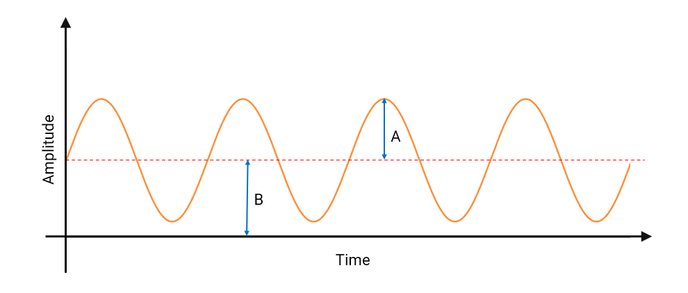
A typical IoT application using a sinusoid is shown below:
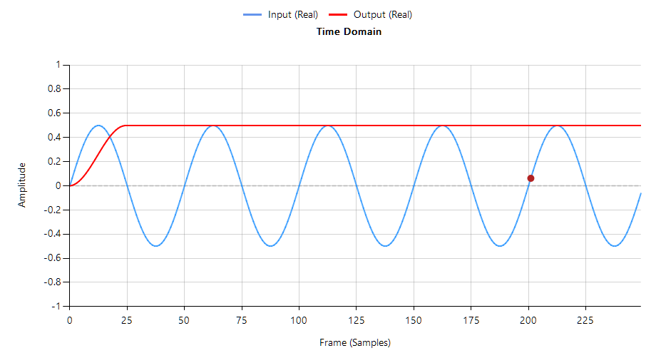
Where, \(f_o\) is the frequency of oscillation and \(A\) is the amplitude of sinusoid respectively. Notice that the sinusoid is non-linear and symmetrical around the offset, \(B\). Notice also that it has a peak-to-peak amplitude of \(2A\), since specifying an amplitude \(A\) results in a bipolar amplitude of \(±A\). As many microcontrollers employ low-cost unipolar ADCs, the bipolar sinusoid needs to be offset by a DC offset, \(B\) (usually achieved by a resistor network) to ensure that the signal remains within the common-mode range of the ADC input.
As mentioned above, before applying the non-linear operator any DC offsets need to be removed. This can easily be achieved with either an IIR or FIR highpass filter. If using an IIR filter, it should be noted that the filter’s phase and group delay (latency) will significantly increase at the cut-off frequency, so a degree of experimentation is required to find a good trade-off.
After highpass filtering the data, we can apply the non-linear operator. Two popular operators are the abs()and sqr()operators.
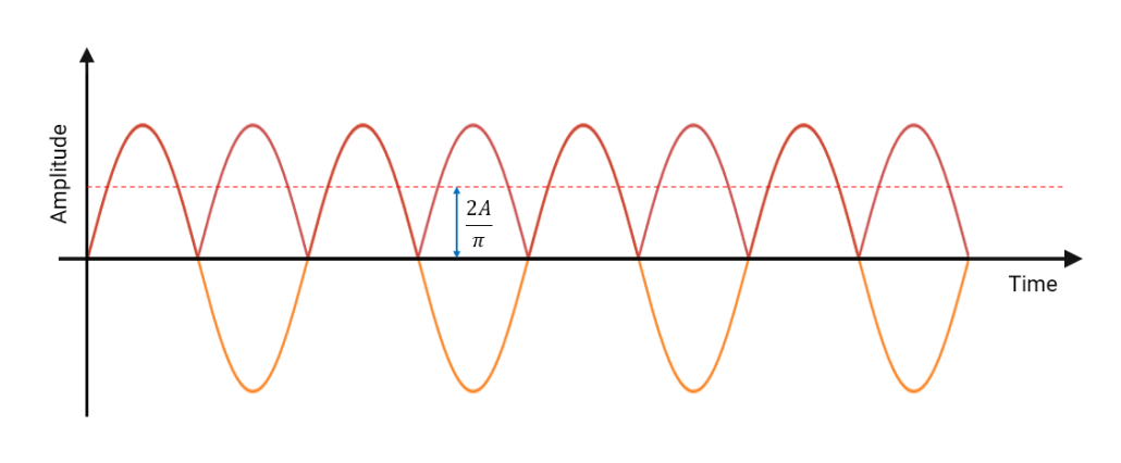
Using the abs()operator, the Fourier series of \(\left|A \,sin(2\pi f_ot)\right|\) is shown below:
Analysing the equation, it can be seen that the abs() operation doubles the frequency and that the DC component is actually \(\frac{2A}{\pi}\), as illustrated below.
As seen, lowpass filtering this result in its current form will produce an amplitude estimate of \(\frac{2A}{\pi}\) (dashed red line), which is clearly incorrect for estimating the sinewave’s amplitude, \(A\). However, this can be simply remedied by scaling the amplitude estimates by \(\frac{\pi}{2}\), which removes the bias, leaving the sinewave’s amplitude, \(A\).
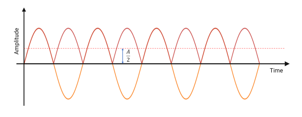
Likewise, for a sqr() operator, we can define the resulting waveform using trigonometrical identities, i.e.
Lowpass filtering this signal requires a correction scaling factor of 2.
Lowpass filter
Although any lowpass filter will suffice, the moving average filter is used by most developers by virtue of its computational simplicity and noise reduction characteristics. A more detailed explanation of moving average filters can be found here.
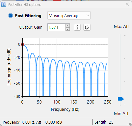
A 24th order moving average filter with a post gain of \(\frac{\pi}{2}\) or 1.571 is shown below.
Applying this moving average filter to a sinewave \(f_o=10Hz, A=0.5\), sampled at 500Hz processed with the abs()operator we obtain the following:
As seen, the amplitude estimation of the sinusoid using a lowpass filter and the \(\frac{\pi}{2}\) scaling factor is now correct. However, for real world applications that contain noise, it is considered to be more accurate to measure the RMS amplitude, in which case the scaling factor becomes \(\frac{\pi}{2\sqrt 2} \).
As a final point, these scaling factors are only valid for sinusoidal scaling. If your waveform is non-sinsoidual (e.g. triangular or square) another scaling factor will be required.
Sanjeev is an AIoT visionary and expert in signals and systems with a track record of successfully developing over 25 commercial products. He is a Distinguished Arm Ambassador and advises top international blue chip companies on their AIoT solutions and strategies for I4.0, telemedicine, smart healthcare, smart grids and smart buildings.
AIoT is an exciting new area that combines AI concepts (i.e. ML) with IoT in order to produce state-of-the-art smart embedded solutions. This augmentation of technologies requires a new set of tools to capture real-time IoT sensor data, analyse it, design suitable algorithms and then perform validation of the solution. After completing validation of the algorithms on the test data, a final hurdle is then how to generate efficient C code of the developed algorithm(s) for an Arm Cortex-M microcontroller for use in an application. These concepts will be discussed herein.
Arm’s Synchronous Data Stream (SDS) Framework provides developers with an easy method of capturing and playing back real-time sensor data for embedded AIoT sensor applications on Arm Cortex-M processors, such as ST Microelectronics’ very popular STM32 family.
The SDS Framework provides embedded developers with a variety of essential tools, such as the ability to record real-world sensor data for analysis and development in tools such as ASN Filter Designer, Python and Matlab. A set of Python utility scripts are available for recording, playback, visualisation and data conversion, where the latter supports the conversion of captured SDS data files into a single CSV file – providing a simple bridge between the ASN Filter Designer and the SDS Framework.
The SDS framework also supports the possibility to playback real-world data for algorithm validation using Arm Virtual Hardware, allowing developers to verify execution of DSP algorithms on Cortex-M targets with off-line tools.
This application note provides AIoT developers with a complete reference guide of how to develop and deploy feature extraction algorithms for use in AIoT applications to STM32 Arm Cortex-M based microcontrollers using STM32CubeIDE or Keil mVision with the Arm SDS framework and ASN Filter Designer. As mentioned above, AIoT system challenges and concepts will also be covered.
Building AIoT systems
Almost all IoT embedded sensor applications require some level of signal processing to enhance sensor data and extract features of interest. However, an obvious hurdle for many developers is how to design, test and deploy efficient algorithms for their application. This is easier said than done, as many software engineers are not well-versed in understanding the mathematical concepts needed to implement algorithms. This is further complicated by the challenge of how to implement algorithms developed by researchers that are not interested/experienced in developing real-time embedded applications.
A possible solution offered by the Mathworks (Embedded Coder) automatically translates Matlab algorithms and functions into C for Arm processors, but its high price tag and steep learning curve make it unattractive for many.
That being said, Arm and its rich ecosystem of partners provide developers with extensive easy-to-use tooling and tried and tested software libraries. Arm’s CMSIS-DSP and CMSIS-NN frameworks for algorithm development and machine learning (ML) are two very popular examples that are open source and are used internationally by tens of thousands of developers.
The Arm CMSIS-DSP software framework is particularly interesting as it provides IoT developers with a rich collection of fast mathematical and vector functions, interpolation functions, digital filtering (FIR/IIR) and adaptive filtering (LMS) functions, motor control functions (e.g. PID controller), complex math functions and supports various data types, including fixed and floating point. The important point to make here is that all of these functions have been optimised for Arm Cortex-M processors, allowing you to focus on your application rather than worrying about optimisation.
The Arm-CMSIS framework solutions are strengthened by Arm partners ASN and Qeexo who provide developers with easy-to-use real-time filtering, feature extraction (ASN Filter Designer) and ML tooling (AutoML) and reference designs, expediting the development of AIoT applications, including industrial, audio and biomedical. These solutions have been optimised for Arm processors with the help of Arm’s architecture experts and insider knowledge of compiler workings.
AIoT system building blocks
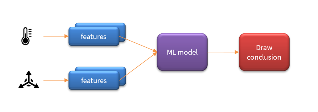
An essential pre-building block in any AIoT system is the feature extraction algorithm. The challenge for any feature extraction algorithm is to extract and enhance any relevant sensor data features in noisy or undesirable circumstances and then pass them onto the ML model in order to provide an accurate classification. The concept is illustrated below:
As seen above, an AIoT system may actually contain multiple feature blocks per sensor and in some cases fuse the features locally before sending them onto the ML model for classification such that the system may then draw a conclusion. The challenge is therefore how to capture sensor data for training and design suitable algorithms to extract features of interest.
Feature extraction algorithms: challenges and solutions
The challenge for any feature extraction algorithm is to extract and enhance any relevant data features in noisy data or undesirable circumstances and then pass them onto the ML model in order to provide an accurate classification. Unfortunately, many ML models perform badly, due to poor quality data and insufficient training data. An obvious challenge for AIoT is how do we obtain the training data in the first place? In many cases, this is extremely challenging as data pertaining to faults (such as preventive maintenance) is hard to come by, as many plant managers are reluctant to break their working production lines or processes to provide developers with training data.
In the absence of adequate training data, feature extraction based on science and mathematics is a prudent alternative, as less training data is required, and in general, the quality of the feature estimate is higher as knowledge of the underlying process is used. Examples include: obtaining accurate pulse and heart rate estimates from ECG and PPG sensors in smartwatch applications when a subject is moving. For industrial sensors, such as loadcells, pressure, temperature, gas and accelerometer sensors the challenge is amplified, as harsh operating conditions and the sheer variety of the applications needed for I4.0 process control applications complicate the design significantly.
Example: Infrared gas sensor
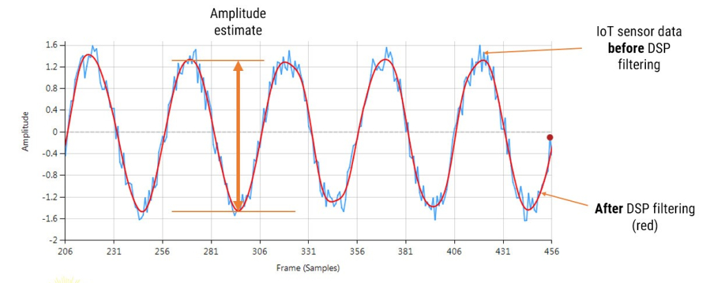
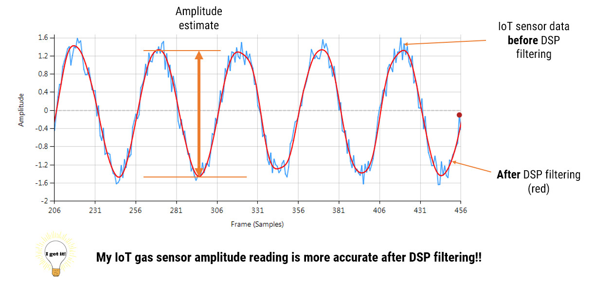
Consider the following application for gas concentration measurement from an Infrared gas sensor. The requirement is to determine the peak-to-peak amplitude of the sinusoid in order to get an estimate of gas concentration – where the bigger amplitude is the higher the gas concentration will be.
Analysing the Figure, it can be seen that the sinusoid is corrupted with measurement noise (shown in blue), and any estimate based on the blue signal will have a high degree of uncertainty about it – which is not very useful for getting an accurate reading of gas concentration! After cleaning the sinusoid with a digital filter (red line), we obtain a much more accurate and usable signal for our gas concentration estimation challenge. But how do we obtain the amplitude?
Knowing that the gradient at the peaks is zero, a relatively easy and robust way of finding the peaks of the sinusoid is via numerical differentiation, i.e. computing the difference between sample values and then looking for the zero-crossing points in the differentiated data. Armed with the positions and amplitudes of the peaks, we can take the average and easily obtain the amplitude and frequency. Notice that any DC offsets and low-frequency baseline wander will be removed via the differentiation operation.
This is just a simple example of how to extract the properties of a sinusoid in real-time using science and mathematics and an understanding of the underlying process without the need for ML training data.
Arm’s Synchronous Data Stream (SDS) Framework provides developers with an easy method of capturing and playing back real-time sensor data for embedded AIoT sensor applications on Arm Cortex-M processors. A set of Python utility scripts are available for recording, playback, visualisation and data conversion, where the latter supports the conversion of captured SDS data files into a single CSV file – providing a simple bridge between the ASN Filter Designer and the SDS Framework.
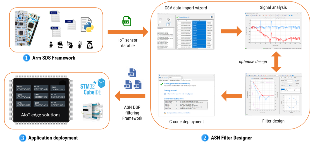
An AIoT smart sensor design workflow using the ASN Filter Designer and the SDS Framework is shown below.
As seen above, three major components constitute the AIoT design workflow.
Arm SDS Framework: capturing IoT sensor data and converting it to CSV format.
ASN Filter Designer: importing the CSV datafile and then analysing the data. Based on the data analysis, a suitable filter can be designed together with other filters and IP blocks in order to build feature extraction algorithms for ML applications.
Application deployment: Generating optimised C code and combining the design with an application for use on an Arm microcontroller.
The SDS Framework can be used with all major demo boards, including ST’s Discovery kit and Nucleo boards. SDS Python utilities are used to convert the captured *.sds and *.yaml files into a CSV file for import into the ASN Filter Designer, as discussed in the following section.
Data Import Wizard
The ASN Filter Designer’s comprehensive data import wizard can delimitate and import a variety of multi-column IoT datasets in CSV or TXT form.
As seen in the video, a generated CSV file can be dragged and dropped onto the signal analyser canvas, bringing up the data import wizard. The import wizard will automatically check the imported data for errors (such as NaNs, Infs etc) and then order the data into columns. Any header line data can be skipped by setting the Skip Headerlines value respectively.
For the example considered herein, the data is actually triaxial accelerometer data (i.e. X, Y and Z axes) with an extra column for the timebase. Therefore, if we wish to import the X-axis data, we can simply click on the header for the second column (B). The tool will then ask you to recheck the data, and upon clicking on ‘Save’ will save the selected data as a single-column CSV file (needed for the ASN Filter Designer). This new CSV file can then be streamed via the tool’s signal generator for algorithm development.
Deploying to Arm Cortex-M processors
After completing the design process, the designed filter(s) can be deployed to STM32CubeIDE or Arm/Keil uVision for integration into an application project. Depending on the functionality of the ASN Filter Designer’s signal chain, two software frameworks are available: Arm’s CMSIS-DSP and ASN’s ANSI C DSP.
The ANSI C DSP framework was developed with close collaboration with Arm’s architecture team, providing outstanding computational performance that is required for real or complex coefficient floating-point designs that use multiple filters and mathematical functions in a signal chain. The Arm CMSIS-DSP framework on the other hand is an excellent choice for implementing both fixed-point and floating-point filters, but is limited to real coefficient single FIR filter or one IIR Biquad cascade with no extra mathematical functions.
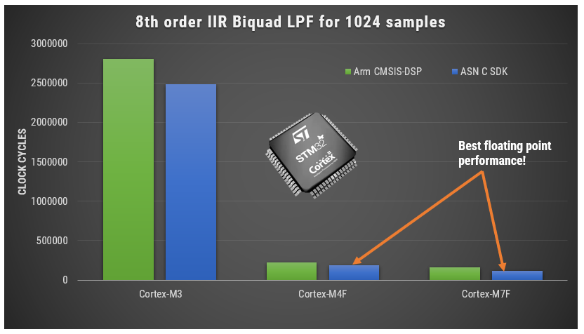
A benchmark comparison for both frameworks is shown below for an 8th IIR filter running on three different Arm cores. As seen, the ASN Framework is slightly faster (lower means better performance) than the Arm Framework.
Framework Benchmarks: lower number of clock cycles means higher performance.
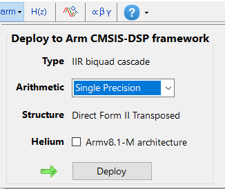
Arm CMSIS-DSP wizard
Professional licence users may expedite the deployment by using the Arm deployment wizard. The tool will automatically analyse your design and choose a suitable Framework. If the design cannot be exported via the Arm CMSIS-DSP framework, the tool will suggest that you use the ASN ANSI C framework and launch the code generation wizard.
Note that the built-in AI will automatically determine the best settings for your design based on the quantisation settings chosen.
Clicking on Deploy will automatically analyse your complete filter cascade and convert any extra filters in the cascade into an H1 (primary) for implementation. Upon completion, the tool will then launch the C code generation wizard.
CMSIS-DSP C code generation
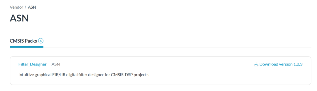
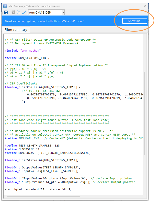
Depending on which C framework is used, the C code generator wizard will automatically generate the C code needed for your design. For developers using the Arm CMSIS-DSP framework, a single C file is generated for use with an MDK5 software pack. The MDK5 pack is available from Arm Keil’s software pack repository, providing several complete filtering examples based on the ASN Filter Designer’s code generator using the Arm CMSIS-DSP library.
A detailed help tutorial is available by clicking on the Show me button.
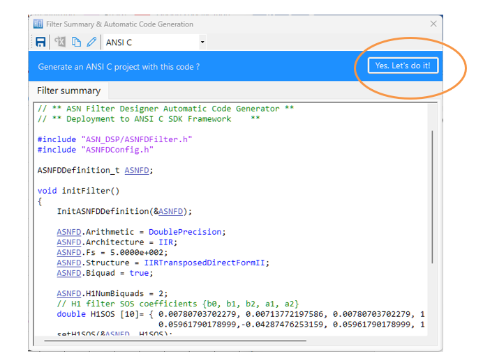
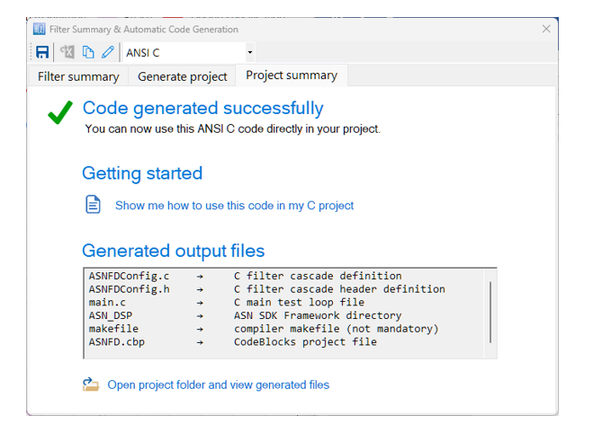
ASN ANSI C DSP code generation
For developers using the ASN ANSI C DSP framework, the code wizard should be used.
NB. The wizard will produce a CodeBlocks project in order to get you started. The following section describes in detail the steps needed for using the generated code in a STM32CUBE-IDE project. Please refer to the ANSI C SDK user guide for step-by-step instructions on how to use the generated code in other IDEs.
A PDF version of this article is available as an application note.
Sanjeev is an AIoT visionary and expert in signals and systems with a track record of successfully developing over 25 commercial products. He is a Distinguished Arm Ambassador and advises top international blue chip companies on their AIoT solutions and strategies for I4.0, telemedicine, smart healthcare, smart grids and smart buildings.
https://www.advsolned.com/wp-content/uploads/2023/07/sds_asnfd.png6431393Dr. Sanjeev Sarpalhttps://www.advsolned.com/wp-content/uploads/2018/02/ASN_logo.jpgDr. Sanjeev Sarpal2023-07-31 11:55:472024-02-16 12:33:52Design of AIoT algorithms with the ASN Filter Designer and the Arm SDS Framework and their deployment to STM32 microcontrollers
Advances in telemedicine healthcare products over the past decades have been truly miraculous with ingenious little devices invented by start-ups as well as by larger corporations, .e.g Apple’s smart watch and the Fitbit. These advancements have been facilitated by the availability of low-cost microcontrollers offering algorithmic functionality, allowing developers to implement wearables with excellent battery life and edge based real-time data analysis.
Over 90% of the microcontrollers used in the smart product market are powered by so called Arm Cortex-M processors that offer a combination of high algorithmic performance, low-power and security. The Arm Cortex-M4 is a very popular choice with hundreds of silicon vendors (including ST, TI, NXP, ADI, Nordic, Microchip, Renesas), as it offers DSP (digital signal processing) functionality traditionally found in more expensive devices and is low-power. Arm and its rich eco system of partners provide developers with easy-to-use tooling and tried and tested software libraries, such as the CMSIS-DSP and CMSIS-NN frameworks for algorithm development and machine learning.
The choice is vast, and can be very confusing. Therefore, here are some practical hints and tips for both managers and developers to help you decide which Arm Cortex-M processor is best for your biomedical product.
Which Arm Cortex-M processor do I choose for my biomedical application?
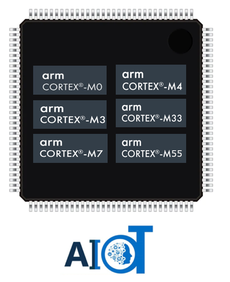
The Arm Cortex-M0+ processor is an ultra-low power 32-bit processor designed for very low-cost IoT applications, such as simple wearable devices. The low price point is comparable with equivalent 8-bit devices, but with 32-bit performance. Microcontrollers built around the M0+ processor provide developers with excellent battery life (months to years), a rich peripheral set and a basic amount of connectivity and computational performance. The latter means that only simple algorithms can be implemented, such as algorithms for correcting baseline wander and minimizing the effects of motion artefacts using accelerometer data via an adaptive filter, such as the NLMS algorithm. Although for PPG pulse rate measurement applications, the sampling rate is typically 50Hz, leaving the processor plenty of time to perform various simpler algorithmic operations, such as digital filtering and zero-crossing detection.
For high performance PPG applications, sampling rates in the order of 500Hz are typically used. These types of applications usually look at more biomedical features, such as identifying the Systolic and Diastolic phases and finding the Dicrotic notch using feature extraction algorithms and ML models. These extra functionalities provide a significant strain on the processor’s abilities, and as such are beyond the abilities of the M0+.
The Cortex-M3 is a step up from the M0+, offering better computational performance but with less power efficiency. The extra processing power, rich hardware peripheral set for connecting other sensors and connectivity options makes the M3 a very good choice for developers looking to develop slightly more advanced wearable products, such as the Fitbit device that is based on ST’s low-power STM32L series of microcontrollers.
High performance wearables and beyond
The Arm Cortex-M4 processor and its more powerful bigger brother the Cortex-M7 are highly-efficient embedded processors designed for IoT applications that require decent real-time signal processing performance and memory. Depending on the flavour of the processor, the M4F/M7F processors implement DSP hardware accelerated instructions, as well hardware floating point support. This lends itself to the efficient implementation of much more computationally intensive biomedical DSP and ML algorithms needed for more advanced telemedicine products.
The hardware floating point support unit expedites RAD (rapid application development), as algorithms and functions developed in Matlab or Python can be ported to C for implementation without the need for a lengthy data arithmetic quantisation analysis. Microcontrollers based on the M4F or M7F, usually offer many of the hardware peripheral and connectivity advantages of the M3, providing developers with a very powerful, low power development platform for their telemedicine application.
The Arm Cortex-M33 is a step up from the M4 focusing on algorithms and hardware security via Arm’s TrustZone technology and memory-protection units. The Cortex-M33 processor attempts to achieve an optimal blend between real-time algorithmic performance, energy efficiency and system security.
State-of-the art AI microcontrollers
Released in 2020, the Arm Cortex-M55 processor and its bigger brother the Cortex-M85 are targeted for AI applications on microcontrollers. These processors feature Arm’s Helium vector processing technology, bringing energy-efficient digital signal processing (DSP) and machine learning (ML) capabilities to the Cortex-M family. In November 2023, Arm announced the release of Cortex-M52 processor for IoT applications. This processor looks to replace the older M33 processor, as it combines Helium technology with Arm TrustZone technology.
Although the IP for these processors is available for licencing, only a few IC vendors have developed a microcontroller, e.g. Samsung’s Exynos W920 SoC that has been specifically designed for the wearables market. The SoC packs two Arm Cortex-A55 processors, and the Arm Mali-G68 GPU using state-of-the art 5nm semiconductor technology. The chipset also features a dedicated low-power Cortex-M55 display processor for handling AoD (Always-on Display) tasks – although a little over the top for simple wearable devices, the Exynos processor family certainly seems like an excellent choice for building next generation AI capable low-power wearable products.
So, which one do I choose?
The compromise for biomedical product developers when choosing an M4, M7 or M33 based microcontroller over an M3 device usually comes down to a trade-off between algorithmic performance, security requirements and battery life. If good battery life and simple algorithms are key, then M3 devices are a good choice. However, if more computationally intensive analysis algorithms are required (such as ML models), then the M4 or M7 should be used.
As mentioned earlier, the Armv7E-M architecture used in M4/M7 processors supports a DSP extension that implements an SIMD (single instruction, multiple data) architecture extension that can significantly improve the performance of an algorithm. The hardware floating point unit is very good for expediting MAC (multiply and accumulate) operations used in digital filtering, requiring just three cycles to complete. Other DSP operations such as add, subtract, multiply and divide require just one cycle to complete.
The M7 out performs its M4 little brother by offering approximately twice the computational performance and some devices even offer hardware double precision floating point support which make M4/M7 processors attractive for high accuracy algorithms needed for medical analysis.
If data security is paramount, for example protecting and securing transferring patient data to a cloud service, then the M33 or the M52 (when avalaible) are good choices. These devices also offer a high level of protection against tampering and running of authorised code via TrustZone’s trusted execution environment.
Some IC vendors now offer hybrid micro-controllers that implement multi-processors on chip, such as ST’s ST32Wx family that combine the M0+ and M4 in order to get the advantages of each processor and maximise battery life.
Finally, advances in semiconductor technology means that a modern M4F processor produced with 40nm process technology may match or even surpass the energy efficiency of an M3 produced with 90nm technology from several years ago. As such, higher performance processors that were until several years too costly and energy inefficient for low-cost wearables products are rapidly becoming a viable solution to this exciting marketplace.
Sanjeev is an AIoT visionary and expert in signals and systems with a track record of successfully developing over 25 commercial products. He is a Distinguished Arm Ambassador and advises top international blue chip companies on their AIoT solutions and strategies for I4.0, telemedicine, smart healthcare, smart grids and smart buildings.
https://www.advsolned.com/wp-content/uploads/2023/04/armcores_biomedical-1.png540865Dr. Sanjeev Sarpalhttps://www.advsolned.com/wp-content/uploads/2018/02/ASN_logo.jpgDr. Sanjeev Sarpal2023-04-19 10:48:562023-12-18 11:45:42Choosing the right Arm Cortex-M processor for your biomedical smart product: a practical guide
We live in a time where wearable/mobile products comprised of sensors, apps, AI and IoT (AIoT) technology are part of everyday life. Every year we hear about amazing advances in processor technology and AI algorithms for all aspects of life from industrial automation to futuristic biomedical products.
For developers, the requirement to design low-cost products with better battery life, higher computational performance and analytical accuracy, requires access to a suite of affordable processor technology, algorithmic libraries, design tooling and support.
This article aims to provide developers with an overview of all salient points required for algorithm implementation on Arm Cortex-M processors.
Can you give me a concrete example?
Almost all IoT sensor applications require some level of signal processing to enhance data and extract features of interest. This could be temperature, humidity, gas, current, voltage, audio/sound, accelerometer data or even biomedical data.
Consider the following application for gas concentration measurement from an Infra-red gas sensor. The requirement is to determine the amplitude of the sinusoid in order to get an estimate of gas concentration – where the bigger amplitude is the higher the gas concentration will be.
Analysing the figure, it can be seen that the sinusoid is corrupted with measurement noise (shown in blue), and any estimate based on the blue signal will have a high degree of uncertainty about it – which is not very useful for getting an accurate reading of gas concentration!
After cleaning the sinusoid with a digital filter (red line), we obtain a much more accurate and usable signal for our gas concentration estimation challenge. But how do we obtain the amplitude?
Knowing that the gradient at the peaks is zero, a relativity easy and robust way of finding the peaks of the sinusoid is via numerical differentiation, i.e. computing the difference between sample values and then looking for the zero-crossing points in the differentiated data. Armed with the positions and amplitudes of the peaks, we can take the average and easily obtain the amplitude and frequency. Notice that any DC offsets and low-frequency baseline wander will be removed via the differentiation operation.
This is just a simple example of how to extract the properties of a sinusoid in real-time using various algorithmic IP blocks. There are of course a number of other methods that may be used, such as complex filters (analytic signals), Kalman filters and the FFT (Fast Fourier Transform).
Arm Cortex-M processor technology
Although a few processor technologies exist for microcontrollers (e.g. RISC-V, Xtensa, MIPS), over 90% of the microcontrollers used in the smart product market are powered by so-called Arm Cortex-M processors that offer a combination of high algorithmic performance, low-power and security. The Arm Cortex-M4 is a very popular choice with several silicon vendors (including ST, TI, NXP, ADI, Nordic, Microchip, Renesas), as it offers DSP (digital signal processing) functionality traditionally found in more expensive devices and is low-power.
Algorithmic libraries and support
An obvious hurdle for many developers is how to port their algorithmic concept or methods from Python/Matlab into embedded C for real-time operation? This is easier said than done, as many software engineers are not well-versed in understanding the mathematical concepts needed to implement algorithms. This is further complicated by the challenge of how to implement algorithms developed by researchers that are not interested/experienced in developing real-time embedded applications.
A possible solution offered by the Mathworks (Embedded Coder) automatically translates Matlab algorithms and functions into C for Arm processors, but its high price tag and steep learning curve make it unattractive for many.
That being said, Arm and its rich ecosystem of partners provide developers with extensive easy-to-use tooling and tried and tested software libraries. Arm’s CMSIS-DSP and CMSIS-NN frameworks for algorithm development and machine learning (ML) are two very popular examples that are open source and are used internationally by tens of thousands of developers.
The Arm CMSIS-DSP software framework is particularly interesting as it provides IoT developers with a rich collection of fast mathematical and vector functions, interpolation functions, digital filtering (FIR/IIR) and adaptive filtering (LMS) functions, motor control functions (e.g. PID controller), complex math functions and supports various data types, including fixed and floating point. The important point to make here is that all of these functions have been optimised for Arm Cortex-M processors, allowing you to focus on your application rather than worrying about optimisation.
The Arm-CMSIS framework solutions are strengthened by Arm partners ASN and Qeexo who provide developers with easy-to-use real-time filtering, feature extraction and ML tooling (AutoML) and reference designs, expediting the development of IoT applications, including industrial, audio and biomedical. These solutions have been optimised for Arm processors with the help of Arm’s architecture experts and insider knowledge of compiler workings.
A benchmark of ASN’s floating point application-specific DSP filtering library versus Arm’s CMSIS-DSP library is shown below for three types of Arm cores.
Framework Benchmarks: lower number of clock cycles means higher performance.
As seen, the performance of the ASN library is slightly faster by virtue of the application-specific nature of the implementation. The C code is automatically generated from the ASN Filter Designer tool.
Cortex-M4 and Cortex-M7
The Arm Cortex-M4 processor and its more powerful bigger brother the Cortex-M7 are highly-efficient embedded processors designed for IoT applications that require decent real-time signal processing performance and memory.
Both the Cortex-M4 and M7 core benefit from the Armv7E-M architecture that offers additional DSP extensions. Depending on the flavour of the processor, the M4F/M7F processors implement DSP hardware accelerated instructions (SIMD), as well as hardware floating point support via an FPU (floating point unit), giving them a significant performance boost over the Cortex-M3. The ‘F’ suffix signifies that the device has an FPU.
This lends itself to the efficient implementation of much more computationally intensive DSP and ML algorithms needed for more advanced IoT products and real-time control applications requiring highly deterministic operations.
Microcontrollers based on the M4F or M7F, usually offer many of the hardware peripheral and connectivity advantages of the simpler M3, providing developers with a very powerful, low-power development platform for their IoT application. The Cortex-M7F typically offers much higher performance than its Cortex-M4F little brother, doubling the performance on FFT, digital filters and other critical algorithms.
Floating point or fixed point?
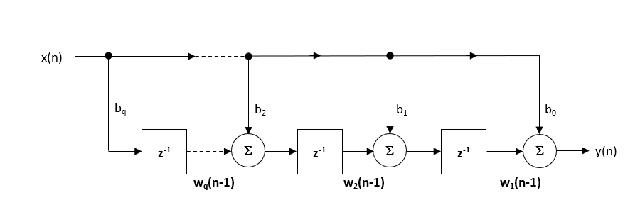
The hardware floating point support unit expedites RAD (rapid application development), as algorithms and functions developed in Matlab or Python can be ported to C for implementation without the need for a lengthy data arithmetic quantisation analysis. Although floating point comes with its own problems, such as numeric swamping, whereby adding a large number to a small number ignores the smaller component. This can become troublesome in digital filtering applications using the standard Direct Form structure. It is for this reason that all floating-point filters should be implemented using the Direct Form Transposed structure, as discussed in the following article.
Correctly designing and implementing these tricks requires specialist knowledge of signal processing and C programming, which may not always be available within an organisation. This becomes even more frustrating when implementing new algorithms and concepts, where the effects of the arithmetic are yet to be determined.
Single vs double precision floating point
For a majority of IoT applications single precision (32-bit) floating point arithmetic will be sufficient, providing approximately 7 significant digits of precision. Double precision (64-bit) floating point provides approximately 15 significant digits of precision, but in truth should only be used in applications that require more than 7 significant digits of precision. Some examples include: FFT based noise cancellation, CIC correction filters and Rogowski coil compensation filters.
Some Cortex-M7F’s (e.g. STM32F769) implement a Double precision FPU providing an extra performance boost to high numerical accuracy IoT applications.
Fixed point
Fixed point is not necessarily less accurate than floating point, but requires much more quantisation analysis, which becomes tricky for signals with a wide dynamic range. As with floating point careful analysis is required, as weird effects can appear due to the level of quantisation used, leading to unreliable behaviour if not properly investigated. It is this challenge that can slow down a development cycle significantly, in some cases taking months to validate a new algorithm.
Many developers have traditionally considered devices without an FPU (e.g., Cortex-M0/M3) as the best choice for low-power battery applications. However, when comparing a modern Cortex-M7 device manufactured using 40nm semiconductor process technology, to that of a ten-year-old Cortex-M3 using 180nm process technology, the Cortex-M7 device will likely have a lower power profile.
Acceleration of DSP calculations
The Armv7E-M architecture supports a DSP extension that implements an SIMD (single instruction, multiple data) architecture extension that can significantly improve the performance of an algorithm. The basic idea behind SIMD involves parallel execution of an instruction (eg. Add, Subtract, Multiply, Divide, Abs etc) on multiple data elements via the use of 64 or 128-bit registers. These DSP extension intrinsics (SIMD optimised instruction) support a variety of data types, such as integers, floating and fixed-point.
The high efficiency of the Arm compiler allows for the automatic dissemination of your C code in order to break it up into SIMD intrinsics, so explicit definition of any DSP extension intrinsics in your code is usually unnecessary. The net result for your application is much faster code, leading to better power consumption and for wearables, better battery life.
What algorithmic operations would use this?
The following examples give an idea of operations that can be significantly speeded up with SIMD intrinsics:
vadd can be used to expedite the calculation of a dataset’s mean. Typical applications include average temperature/humidity readings over a week, or even removing the DC offset from a dataset.
vsub can be used to expedite numerical differentiation in peak finding, as discussed in the example above.
vabs can be used for expediting the calculation of an envelope of a fullwave rectified signal in EMG biomedical and smartgrid applications.
vmul can be used for windowing a frame of data prior to FFT analysis. This is also useful in audio applications using the overlap-and-add method.
The hardware floating point unit is very good for expediting MAC (multiply and accumulate) operations used in digital filtering, requiring just three cycles to complete. Other DSP operations such as add, subtract, multiply and divide require just one cycle to complete.
Combining DSP, low-power and security: The Cortex-M33
The Arm Cortex-M33 is based on the Armv8-M architecture and is a step up from the Cortex-M4 focusing on algorithms and hardware security via Arm’s TrustZone technology and memory-protection units. The Cortex-M33 processor attempts to achieve an optimal blend between real-time algorithmic performance, energy efficiency and system security.
TrustZone technology
Arm TrustZone implements a security paradigm that discriminates between the running and access of untrusted applications running in a Rich Execution Environment (REE) and trusted applications (TAs) running in a secure Trusted Execution Environment (TEE). The basic idea behind a TEE is that all TAs and associated data are secure as they are completely isolated from the REE and its applications. As such, this security model provides a high level of security against hacking, stealing of encryption keys, counterfeiting, and provides an elegant way of protecting sensitive client information.
State-of-the art AI microcontrollers
Released in 2020, the Arm Cortex-M55 processor and its bigger brother the Cortex-M85 are targeted for AI applications on microcontrollers. These processors feature Arm’s new Helium vector processing technology based on the Armv8.1-M architecture that brings significant performance improvements to DSP and ML applications. However, as only a few IC vendors (Alif, Samsung, Renesas, HiMax, Bestechnic, Qualcomm) have currently released or are planning to release any devices, Helium processors remain a gem for the future.
Key takeaways
Arm and its rich ecosystem of partners provide IoT developers with extensive easy-to-use tooling and tried and tested software libraries for designing an implementing IoT algorithms for their smart products. Arm Cortex-MxF processors expedite RAD by virtue of their ease of use and hardware floating-point support, and modern semiconductor technology ensures low-power profiles making the technology an excellent fit for IoT/AIoT mobile/wearables applications.
Sanjeev is an AIoT visionary and expert in signals and systems with a track record of successfully developing over 25 commercial products. He is a Distinguished Arm Ambassador and advises top international blue chip companies on their AIoT solutions and strategies for I4.0, telemedicine, smart healthcare, smart grids and smart buildings.
Recent research suggests that ECG wearables devices (such as smart watches) are now medically suitable for providing predictive insights into serious heart conditions such as atrial fibrillation (A-Fib). These advancements have been facilitated by the availability of low-cost microcontrollers offering algorithmic functionality, allowing developers to implement wearables with excellent battery life and edge-based real-time data analysis.
Although the international research community has produced many innovative high-performance ECG and PPG biomedical algorithms, these are unfortunately limited to offline clinical analysis in Matlab or Python. As such, very little emphasis has been placed on building commercial real-time wearables algorithms on microcontrollers, leading manufacturers to conduct the research themselves and to design suitable candidates.
This is further complicated by the requirement of manufacturers on how they will implement a developed algorithm in real-time on a low-cost microcontroller and still achieve decent battery life.
Arm Cortex-M microcontrollers
Over 90% of the microcontrollers used in the smart product market are powered by so-called Arm Cortex-M processors that offer a combination of high algorithmic performance, low-power and security. The Arm Cortex-M4 is a very popular choice with hundreds of silicon vendors (including ST, TI, NXP, ADI, Nordic, Microchip, Renesas), as it offers DSP (digital signal processing) functionality traditionally found in more expensive devices and is low-power.
The Cortex-M4F device offers floating point support, helping with RAD (rapid application development) as designs can be easily ported from Matlab/Python to C without the need of performing a detailed quantisation arithmetic analysis. As such, a design cycle can be cut from months to weeks, offering organisations a significant cost saving.
Arm and its rich ecosystem of partners provide developers with easy-to-use tooling and tried and tested software libraries, such as the CMSIS-DSP and CMSIS-NN frameworks and ASN’s DSP filtering library for algorithm development and machine learning.
FDA compliance
The AHA (American Heart Association) provides developers with guidelines for developing FDA-compliant ECG monitoring products. These are broken down into the following three categories:
Diagnostic: 0.05Hz -150Hz
Ambulatory (wearables): 0.67Hz – 40Hz
ST segment: 0.05Hz
The ECG measurements must be FDA compliant with IEC 60601-2 2-47 standardsfor ambulatory ECG, but what are the criteria and challenges?
Challenges with ECG/PPG measurements
Modelling the QRS complex found in ECG data is extremely difficult, as to date there is no concrete model available. This is further complicated by the variety of ECG data depending on the position of the lead on the patient’s body and illnesses. The following list summaries the typical challenges faced by algorithm developers:
Accurate baseline wander (BLW) removal remains one of the most challenging topics in ECG analysis.
The BLW must be removed for accurate clinical analysis.
BLW manifests itself as low-frequency ‘wander’ (typically <0.5Hz) from EMG and torso movement.
QRS width widening and amplitude distortion due to filtering invalidates clinical analysis.
Reducing EMG and measurement noise without altering the temporal biomedical relationships of the ECG signal.
50/60Hz powerline interference can swamp the ECG signal – this is primarily attributed to pickup by the long high impedance measurement cables. This is typically problematic for extended bandwidth wearable applications that go beyond 40Hz.
Glitches, sudden movement and poor sensor contact with the skin: This is related to BLW, but usually manifests itself as abrupt glitches in the ECG measurement data. The correction algorithm must discriminate between these undesirable events and normal behaviour.
IEC 60601-2 2-47 frequency response specifications:
Bandwidth: 0.67Hz – 40Hz.
Passband ripple: < ±0.5dB
Maximum ±10% amplitude error: most biomedical SoCs make use of a Sigma-Delta ADC, leading to amplitude droop.
Shortcomings with ECG/PPG algorithms
A mentioned in the previous section, much research has been conducted over the years with mixed results. The main shortcomings of these methods are summarised below:
Computationally heavy: most algorithms have been designed for research in Matlab and not for real-time, e.g. wavelets have excellent performance but have high computational cost, leading to poor battery life and the need for an expensive processor.
Large latencyand warping: digital filtering chain introduces large latency, computational cost and can warp the characteristics of the biomedical features.
Overlapping frequencies: there are many examples of unwanted noise overlapping the delicate ECG data, hence the popularity of time-frequency analysis, such as wavelets.
Mixed results regarding BLW removal: spline removal is excellent, but it has high computational cost and has the added difficulty of finding good correction points between the QRS complexes. Linear phase FIR filtering is a good compromise but has very high computational cost (typically >1000 filter coefficients) due to the high sampling rate to cut-off frequency ratio. Non-linear phase IIR filter has low computational cost, but warps the ECG features, and is therefore unsuitable for clinical analysis.
AI based kernel filters: ‘black box filter’ based on massive training data. Moderate implementation cost with performance dependent on the variety of training data, leading to unpredictable results in some cases.
PPG analysis: has the added difficulty of eliminating motion from the measurement data, such as when walking or running. Although a range of tentative algorithms has been proposed by various researchers using accelerometer measurement data to correct the PPG data, very few commercial solutions are currently based on this technology.
It would seem that ECG and PPG analysis has some major obstacles to overcome, especially when considering how to deploy the algorithms on low-power microcontrollers.
The future: ASN’s real-time RCF algorithm and Advanced Analytics
Together with cardiologists from Medisch Spectrum Twente, ASN’s advanced analytics team developed the RCF (retrospective collaborative filtering) algorithm that uses time-frequency analysis to enhance the ECG data in real-time.
The essence of RCF algorithm centres around a highly optimised set of polynomial cleaning filters with different frequency characteristics that are applied to different segments of the QRS complex for enhancement. This has some synergy with wavelets, but it does not suffer from the computational burden associated with wavelet analysis.
The polynomial filters are peak preserving, meaning that they preserve the delicate biomedical peaks while smoothing out the unwanted noise/ripple. The polynomial fitting operation also overcomes the challenge of overlapping frequency content, as data within a specified region is smoothed out by the relevant filter.
RCF is further strengthened by the BLW killer IP block that implements a highly computationally efficient linear phase 0.67Hz highpass filter. The net effect is an FDA-compliant signal chain suitable for clinical analysis. The complete signal chain is extremely computationally efficient, and as such is suitable for Arm’s popular M3 and M4 Cortex-M processor families.
Real-time ECG feature extraction
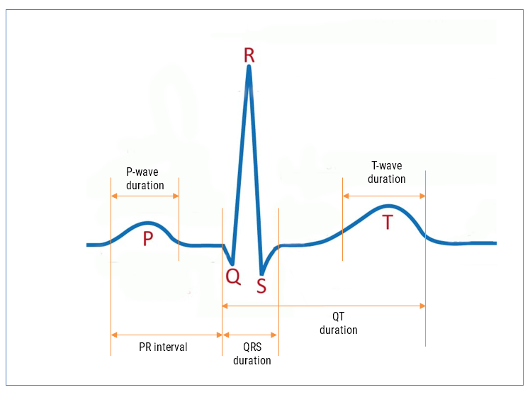
The ECG waveform can be split up into segments, where each wave or segment represents a certain event in the cardiac cycle, as shown below:
As seen, the biomedical features are designated P, Q, R, S, T that define points in time within the cardiac cycle. The RCF algorithm is further strengthened with our state-of-the-art AAE (Advanced Analytics Engine) that automatically cleans and find these features for clinical analysis.
AAE supported analytics
P-wave duration
PR interval
QRS duration
QT duration (Bazett algorithm used for QTc)
HR (RR interval)
HRV (rMSSD algorithm used)
Armed with the real-time features, an ML model can be trained and provide valuable insights into patient health running on an edge processor inside a wearable device.
A-Fib
Atrial fibrillation (A-Fib) is the most frequent cardiac arrhythmia, affecting millions of people worldwide. An arrhythmia is when the heart beats too slowly, too fast, or in an irregular way. Signs of A-Fib are an irregular beating pattern and no p-waves. Our AAE provides developers with all of the relevant features needed to build an ML model for robust A-Fib detection.
Let us help you build your product
By combining advanced low-power processor technology, advanced mathematical algorithmic concepts and medical knowledge, our solution provides developers with an easy way of building wearable products for medical use. The high accuracy of our Advanced Analytics Engine (AAE) has been verified by cardiologists, and can be used with an additional ML model or standalone to provide people with valuable insights into potentially fatal health conditions, such as A-Fib without the need for an expensive medical examination at a hospital.
ASN’s ECG algorithmic solutions are ideal for building next generation ECG and PPG wearable products on Arm Cortex-M microcontrollers (e.g. STM32F4, MAX32660) and bio-sensor SoCs (MAX86150). These algorithms can be easily used with industry standard biomedical AFEs, such as: MAX30003, AFE4500 and AFE4950.
Please contact us for more information and to arrange an evaluation.
Sanjeev is an AIoT visionary and expert in signals and systems with a track record of successfully developing over 25 commercial products. He is a Distinguished Arm Ambassador and advises top international blue chip companies on their AIoT solutions and strategies for I4.0, telemedicine, smart healthcare, smart grids and smart buildings.
Unexpected equipment failures can be expensive and potentially catastrophic, resulting in unplanned production downtime, costly replacement of parts and safety and environmental concerns. With many factories and process control plants facing an ever-increasing shortage of experienced personnel, many are now looking for AI based systems to replace the ‘experienced old guy’ who knows everything about the machine and reduce their Total Cost of Ownership (TOC).
The challenge is however, how do you build and train an AI CbM system to replace an expert ?
What is CbM?
As part of the I4.0 revolution, Condition based monitoring (CbM) of machines has received a great amount of attention, as factories look to maximise their production efficiency and reduce their TOC, while at the same time retaining the invaluable skills of experienced foremen and production workers. As such, CbM is a process for monitoring equipment during operation to identify any deterioration, enabling maintenance to be planned and operational costs reduced.
CbM 5G edge computing
Many are factory owners are suspicious of cloud-based enterprise solutions offered by Microsoft, Amazon and Google as data leaves the site and any latency issues could affect production output. Recently 5G edge computing has received much attention, whereby all time-critical operations are undertaken at the edge (i.e. near to the asset in the factory) via smart sensors.
Arm’s rich set of Cortex processors offer a combination of high performance, ML/DSP computation support and low power. This is further strengthened by Arm’s new Helium Cortex-M55 and Cortex-M85 AI based processors that have been specially designed for edge-based AI applications – the latter offers an impressive 3DMIPS/MHz making it a good fit for ML and DSP algorithms. These processors and supporting libraries now allow developers to develop high-performance CbM smart sensors to perform their computationally intensive tasks at the edge and communicate the results via a 5G network to a smartphone or database. This provides higher reliability and scalability than expensive cloud-based solutions reliant on big data.
It would seem that big data has had its day!
Vibration sensor technology
Contactless MEMS (microelectromechanical systems) accelerometers sensors are an excellent alternative to the well-established, but bulky and expensive (25-500+ EUR) Piezo sensors for obtaining vibration information. MEMS sensors are relatively low cost (10-30 EUR) and can offer a response down to DC (zero Hertz), which is useful for the detection of imbalance at very low rotational speeds. MEMS accelerometers also have a self-test feature whereby the sensor can be verified to be 100% functional. They produce acceleration data that can be analysed by various vibration monitoring algorithms.
Spectral vibration monitoring via the FFT (Fast Fourier Transform) is regarded as an industry standard for machine vibration analysis. If a mechanical problem exists, the FFT spectra (multiple spectrums) will provide information to help determine the source and cause of the problem. Coupled with the right AI algorithms, the features from the FFT analysis can be used to identify the root cause of the failure, such as motor imbalance, misalignment, and looseness. These properties and challenges faced by the FFT will be discussed further later on in the article.
There are several steps to follow as guidelines to help achieve a successful vibration monitoring programme. The following is a general list of these steps:
Collect useful information: Look, listen and feel the machinery to check for resonance. Identify what measurements are needed (point and point type). Conduct additional testing if further data are required.
Analyse spectral data: Evaluate the overall values and specific frequencies corresponding to machinery anomalies. Compare overall values in different directions and current measurements with historical data.
Multi-parameter monitoring: Use additional techniques to conclude the fault type. (Analysis tools such as phase measurements, current analysis, acceleration enveloping, oil analysis and thermography can also be used.)
Perform Root Cause Analysis (RCA): In order to identify the real causes of the problem and to prevent it from occurring again.
Reporting and planning actions: Use a Computer Maintenance Management System (CMMS) to rectify the problem and take action to achieve a plan.
As aforementioned, a popular device used to obtain acceleration data is a so-called ‘accelerometer’. These devices are semiconductor-based MEMS (microelectromechanical systems) and provide 3D (i.e. tri-axial) acceleration time domain data to a supporting microcontroller.
Before FFT analysis, the accelerometer data is usually passed through integration signal processing blocks, in order to convert the time domain acceleration data into velocity and displacement data. These blocks are comprised of a highpass filter and cumulative sum (integration). The highpass filter is essential for removing the effects of DC and noise, which would cause an offset in the output (i.e. the result of the integration). Depending on the severity of the noise/DC the output may even saturate, making it unusable for analysis. The design of a suitable highpass filter is an extremely challenging task and is the primary reason why many vibration analysis systems struggle to measure vibrations <10Hz (600 RPM).
Collect useful information
When conducting a vibration program, certain preliminary information is needed in order to conduct an analysis. The identification of components, running speed, operating environment and types of measurements should be determined initially to assess the overall system.
Identify components of the machine that could cause vibration
Before a spectrum can be analysed, the components that cause vibration within the machine must be identified. For example, you should be familiar with these key components:
If the machine is connected to a fan or pump, it is important to know the number of fan blades or impellers.
If bearings are present, know the bearing identification number or its designation.
If the machine contains, or is coupled, to a gearbox, know the number of teeth and shaft speeds.
If the machine is driven with belts, know the belt lengths.
The above information helps assess spectral components and helps identify the vibration source. Determining the running speed is the initial task. There are several methods to help identify this parameter.
Identifying the running speed
Knowing the machine’s running speed is critical when analysing an FFT spectrum. Running speed is related to most components within the machine and therefore, aids in assessing overall machine health. There are several ways to determine running speed:
Read the speed from instrumentation at the machine or from instrumentation in the control room monitoring the machine.
Look for peaks in the spectrum at 1,800 or 3,600 RPM (60Hz countries), 1,500 and 3,000 RPM (50Hz countries) if the machine is an induction electric motor, as electric motors usually run at these speeds. If the machine is variable speed, look for peaks in the spectrum that are close to the running speed of the machine during the time at which the data is captured.
An FFT’s running speed peak is typically the first significant peak in the spectrum when reading the spectrum from left to right. Search for this peak and check for peaks at two times, three times, four times, etc. (at the harmonic frequencies).
Challenges with the FFT algorithm
FFT spectra allow us to analyse vibration amplitudes at various component frequencies on the FFT spectrum. In this way, we can identify and track vibration occurring at specific frequencies. Since we know that particular machinery problems generate vibration at specific frequencies, we can use this information to diagnose the cause of excessive vibration.
Challenges with spectral analysis
The sampling rate of the accelerometer drifts with temperature: This results in a mismatch between the FFT analysis sampling frequency and the real situation. As such, the amplitude and frequency estimates of the vibration will be incorrect.
Frequency resolution: the frequency of the vibration peak may have a fractional value. If the resolution of the Fourier algorithm is not fine enough, it will ‘smear’ the result, resulting in a lower amplitude estimate.
Running speed: this is typically known apriori, but will have a degree of error associated with it and will change with temperature. For example, 3000 rpm ±1% is 50Hz ±0.5Hz at the fundamental running frequency. In order to track higher harmonics (i.e. multiples of the running speed) the FFT must have sufficient frequency resolution to accurately estimate the amplitude at the right frequency.
Traditional FFT based analysis uses a very high number of computational points in order to achieve a 1Hz resolution. Although this is OK, it still does not overcome the fractional frequency components and requires considerable computational effort.
Some designs use a phaselocked loop, that tracks the running frequency and sets the FFT analysis sampling frequency to a multiple (e.g. 20x) of the running speed. Although this is a very good workaround, it requires specialised hardware (such as an expensive ASIC) and is inflexible for changes in running speed.
ML feature extraction, DSP algorithms and models
In order to build an ML (machine learning) model for an AI CbM application, several challenges need to be overcome.
Definition of classes: In order to make a classification, ML classes must be defined. In the simplest sense, this can be Fault or Normal behaviour, but what about other cases?
ML Features: what data features will be used for the ML model? Running speed, harmonics, RMS amplitude? What physical and mathematical principles should I use to build these algorithms?
Obtaining ML training data: How will you obtain suitable datasets for ML training? In many cases this is not easy to obtain, as many foremen will not allow any disruption to their time-critical production lines.
Preparing datasets: After answering the aforementioned questions, the next challenge will be to capture and prepare the datasets for the ML classification. This is traditionally where a good 90% of a data scientist’s time will be spent. Therefore, it is prudent to invest in high fidelity feature extraction edge algorithms in order to expedite this step. This will also have the advantage of increasing the reproducibility and consistency of the results, which is where many AI based systems perform poorly.
ASN’s IP blocks and applications
ASN’s vibration IP blocks combine the Fourier transform’s time-frequency integration property, data filtering and a specialised high frequency resolution tracking algorithm to implement the ARAHTA (adaptive running speed and harmonics tracking) algorithm. ARAHTA tracks the vibration sensor’s ODR (output data rate) and calculates the motor/pumps running speed using the sensor’s accelerometer sensor data in real-time. ARAHTA’s high resolution and adaptive tracking mechanism results in a typical running speed accuracy of ±1 RPM across the temperature range and sub-mm displacement accuracy using noisy accelerometer data.
ARAHTA’s high accuracy and flexibility ensures that the resulting ML features are high quality and very consistent in the presence of temperature change and load shifts. This has a significant advantage for CbM applications, whereby fingerprinting a spectral profile can be used to assess the degradation of assets of interest. ARAHTA’s high-resolution spectrum forms the basis of providing an AI algorithm with high accuracy feature-rich information, suitable for classification.
Algorithmic performance
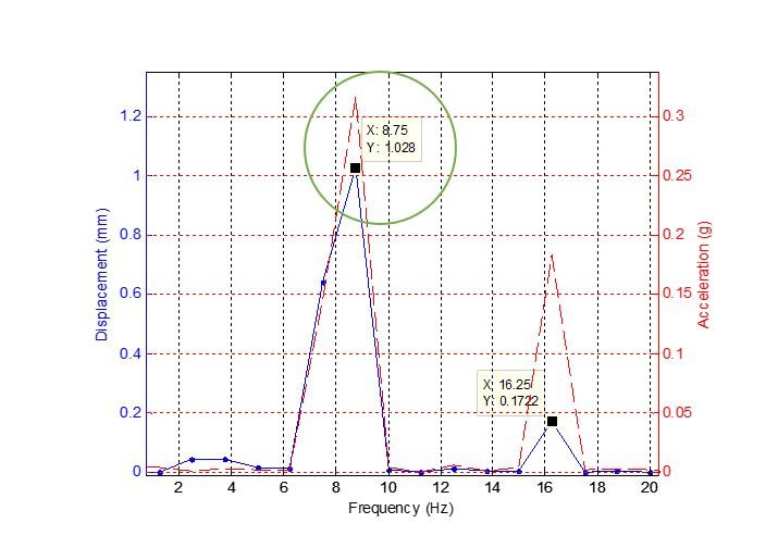
A comparison of the FFT vs the ASN ARAHTA IP blocks is shown below. Setting up a test accelerometer signal comprised of an 8.2Hz sinusoid with amplitude 1gand a few harmonic frequencies at various amplitudes, we can objectively compare the methods.
Analysing Figure 1, notice that the plot shows a comparison of the acceleration spectrum (i.e. the FFT of the acceleration data, shown in red) and the displacement spectrum, shown in blue. Analysing the first peak, notice that as the FFT’s resolution is insufficient, as the algorithm has identified the peak at 8.75Hz, rather than at 8.2Hz. This has a consequence for the amplitude estimation, as the acceleration spectrum amplitude is around 0.34g, rather than the expected 1g. As such, the algorithm incorrectly estimates the displacement at 8.2Hz to be 1mm, rather than 3.69mm.
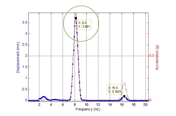
The true value can be seen in Figure 2, where ARAHTA correctly finds the first resonant peak at 8.2Hz and estimates the correct amplitude of 3.69mm.
Figure 1 – Displacement estimate via FFT (frequency resolution: 813.5mHz): wrong frequency and amplitude estimation
Figure 2 – Displacement estimate via ARAHTA (frequency resolution: 10mHz): correct amplitude and frequency estimation.
Get in touch and reduce your asset’s TCO
ASN contactless measurement sensor technology and smart algorithms are an ideal solution for AI based CbM applications. Please contact our CbM expert team to see how we can help you create an effective maintenance programme and reduce your asset’s Total Cost of Ownership.
Sanjeev is an AIoT visionary and expert in signals and systems with a track record of successfully developing over 25 commercial products. He is a Distinguished Arm Ambassador and advises top international blue chip companies on their AIoT solutions and strategies for I4.0, telemedicine, smart healthcare, smart grids and smart buildings.
https://www.advsolned.com/wp-content/uploads/2019/12/induction-motor-1500-580-4_compres2.jpg5801500Dr. Sanjeev Sarpalhttps://www.advsolned.com/wp-content/uploads/2018/02/ASN_logo.jpgDr. Sanjeev Sarpal2022-03-02 17:47:312023-05-12 09:23:54Deploying AI based CbM applications: challenges and algorithmic solutions
ASN Filter Designer’s new ANSI C SDK framework, provides developers with a comprehensive automatic C code generator for microcontrollers and embedded platforms. This allows developers to directly deploy their AIoT filtering application from within the tool to any STM32, Arduino, ESP32, PIC32, Beagle Bone and other Arm, RISC-V, MIPS microcontrollers for direct use.
Arm’s CMSIS-DSP library vs. ASN’s C SDK Framework
Thanks to our close collaboration with Arm’s architecture team, our new ultra-compact, highly optimised ANSI C based framework provides outstanding performance compared to other commercial DSP libraries, including Arm’s optimised CMSIS-DSP library.
Benchmarks for STM32: M3, M4F and M7F microcontrollers running an 8th order IIR biquad lowpass filter for 1024 samples
As seen, using o1 complier optimisation, our framework is able to surpass Arm’s CMSIS-DSP library’s performance on an M4F and M7F. Although notice that performance of both libraries is worse on the Cortex-M3, as it doesn’t have an FPU. Despite the difference, both libraries perform equally well, but the ASN DSP library has the added advantage of extra functionality and being platform agnostic, making it ideal for variety of biomedical (ECG, EMG, PPG), audio (sound effects, equalisers) , IoT (temperature, gas, pressure) and I4.0 (flow measurement, vibration analysis, CbM) applications.
AIoT applications designed on the newer Cortex-M33F and Cortex-M55F cores can also take advantage of extra filtering blocks, double precision arithmetic support, providing a simple way of implementing high performance AI on the Edge applications within hours.
Advantages for developers
A developer can now develop, test and deploy a complete DSP filtering application within the ASN Filter Designer within a few hours. This is very different from a traditional R&D approach that assigns a team of developers for several days in order to achieve the same level of accuracy required for the application.
Open source and agnostic code base: In order to allow developers to get the maximum performance for their applications, the ASN-DSP SDK is provided as open source and is written in ANSI C. This means that any embedded processor and any level of compiler optimisation can be used.
Memory size required for the ASN-DSP SDK is relativity lower than other standard DSP libraries, which makes the ASN-DSP SDK extremely suitable for microcontrollers that have memory constrains.
Using the ASN Filter Designer’s signal analyser tool, developers now can test the performance, accuracy and assess the frequency response of their designed filter and get optimised C code which they can directly use in their application.
The SDK also supports some extra filtering functions, such as: a median filter, a moving average filter, all-pass, single section IIR filters, a TKEO biomedical filter, and various non-linear functions, including RMS, Abs, Log and Sqrt. These functions form the filter cascade within the tool, and can be used to build signal processing applications, such as EMG and ECG biomedical applications.
The ASN-DSP SDK supports both single and double precision floating point arithmetic, providing excellent numerical accuracy and wide dynamic range. The library is unique in the sense that it supports double precision arithmetic, which although is not the most optimal for microcontrollers, allows for the implementation of high-fidelity filtering applications.
The ANSI C SDK framework is further extended by our new C# .NET framework, allowing .NET developers to build high performance desktop applications with signal processing capabilities.
Find out more and try it yourself
Benchmarks on a variety of 32-bit embedded platforms, including a biomedical EMG filtering example, are covered in the following application note.
The both framework SDKs are available in ASNFD v5.0, which may be downloaded here.
Drones are one of the golden nuggets in AIoT. No wonder, they can play a pivotal role in congested cities and faraway areas for delivery. Further, they can be a great help to give an overview of a large area or for places which are difficult or dangerous to reach. Advanced Solutions did some research how the companies producing drones has solved some questions regarding their sensor technology. And in drones, there are a lot of sensors- and especial the DC motor control. We found out that with ASN Filter Designer, producers could have saved time and energy in the design of their algorithms with ASN Filter Designer.
Until now: hard-by found solutions
We found out that most producers had come very hard-by to their solutions. And that, when solutions are found, they are far from near perfect.
Probably, this producer has spent weeks or even months on finding these solutions. With ASN Filter Designer, he could have come to a solution within days or maybe hours. Besides, we expect that the measurement would be better too.
The most important issue is that algorithms were developed by handwork: developed in a ‘lab’ environment and then tried in real-life. With the result of the test, the algorithm would be adjusted again. Because a ‘lab’ environment where testing circumstances are stable, it’s very hard work to make the models work in ‘real’ life. For this, rounds and rounds of ‘lab development’ and ‘real life testing’ have to be made.
How ASN Filter Designer could have saved a lot of time and energy
ASN Filter Designer could have saved a lot of time in the design of the algorithms the following ways:
Design, analyze and implement filters for Drone senor applications
Filters for speed and positioning control using sensorless BLDC motors
Speed up deployment
Real-time feedback and powerful signal analyzer
One of the key benefits of the ASN Filter Designer and signal analyzer is that it gives real-time feedback. Once an algorithm is developed, it can easily be tested on real-life data. To capture the real-life data, the ASN Filter Designer has a powerful signal analyzer in place. The tool’s signal analyzer implements a robust zero-crossings detector, allowing engineers to evaluate and fine-tune a complete sensorless BLDC control algorithm quickly and simply.
Design and analyze filters the easy way
You can easily design, analyze and implement filters for drone sensor applications. Including: loadcells, strain gauges, torque, pressure, temperature, vibration and ultrasonic sensors. And assess their dynamic performance in real-time with different input conditions. With the ASN Filter Designer, no algorithms are needed: you just have to drag the filter design. The tool calculates the coordinates itself.
For speed and position control using sensorless BLDC (brushless DC) motors based on back-EMF filtering you can easily experiment with the ASN Filter Designer. See the results in real-time for various IIR, FIR and median (majority filtering) digital filtering schemes. The tool’s signal analyzer implements a robust zero-crossings detector. So you can evaluate and fine-tune a complete sensorless BLDC control algorithm quickly and simply.
Speed up deployment
Perform detailed time/frequency analysis on captured test datasets and fine-tune your design. Our Arm CMSIS-DSP and C/C++ code generators and software frameworks speed up deployment to a DSP, FPGA or micro-controller.
Drones use lots of sensors, and most challenges will be solved with them! ASN Filter Designer provides you with a simple way of improving your sensor measurement performance with its interactive design interface.
So, if you have a measurement problem, ask yourself: will I have a lot of frustrating and costs (maybe not ‘out of pocket’, but still: costs) of creating a filter by hand? Or would I create my filter within days or even hours and save a lot of headache and money. Because: it’s already possible to have a full 3-month license for only 140 euro!
https://www.advsolned.com/wp-content/uploads/2018/07/droneengineers-1.jpg4781300ASN consultancy teamhttps://www.advsolned.com/wp-content/uploads/2018/02/ASN_logo.jpgASN consultancy team2021-07-07 10:22:522022-12-13 16:06:09Save time and energy in the design of the algorithms for Drones and DC motor control with ASN Filter Designer
The global smart sensor market size is projected to grow from USD 36.6 billion in 2020 to USD 87.6 billion by 2025, at a CAGR of 19.0%. At least 80% of these IoT/IIoT smart sensors (temperature, pressure, gas, image, motion, loadcells) will use Arm’s Cortex-M technology.
IoT sensor measurement challenge
The challenge for most, is that many sensors used in these applications require filtering in order to clean the measurement data in order to make it useful for analysis.
Let’s have a look at what sensor data really is…. All sensors produce measurement data. These measurement data contain two types of components:
Wanted components, i.e. information what we want to know
Unwanted components, measurement noise, 50/60Hz powerline interference, glitches etc – what we don’t want to know
Unwanted components degrade system performance and need to be removed.
So, how do we do it?
DSP means Digital Signal Processing and is a mathematical recipe (algorithm) that can be applied to IoT sensor measurement data in order to clean it and make it useful for analysis.
But that’s not all! DSP algorithms can also help:
In analysing data, producing more accurate results for decision making with ML (machine learning)
They can also improve overall system performance with existing hardware. So ther’s no need to redesign your hardware: a massive cost saving!
To reduce the data sent off to the cloud by pre-analysing data. So send only the data which is necessary
Nevertheless, DSP has been considered by most to be a black art, limited only to those with a strong academic mathematical background. However, for many IoT/IIoT applications, DSP has been become a must in order to remain competitive and obtain high performance with relatively low cost hardware.
Do you have an example?
Consider the following application for gas sensor measurement (see the figure below). The requirement is to determine the amplitude of the sinusoid in order to get an estimate of gas concentration (bigger amplitude, more gas concentration etc). Analysing the figure, it is seen that the sinusoid is corrupted with measurement noise (shown in blue), and any estimate based on the blue signal will have a high degree of uncertainty about it – which is not very useful if getting an accurate reading of gas concentration!
Algorithms clean the sensor data
After ‘cleaning’ the sinusoid (red line) with a DSP filtering algorithm, we obtain a much more accurate and usable signal. Now we are able to estimate the amplitude/gas concentration. Notice how easy it is to determine the amplitude of red line.
This is only a snippet of what is possible with DSP algorithms for IoT/IIoT applications, but it should give you a good idea as to the possibilities of DSP.
How do I use this in my IoT application?
As mentioned at the beginning of this article, 80% of IoT smart sensor devices are deployed on Arm’s Cortex-M technology. The Arm Cortex-M4 is a very popular choice with hundreds of silicon vendors, as it offers DSP functionality traditionally found in more expensive DSPs. Arm and its partners provide developers with easy to use tooling and a free software framework (CMSIS-DSP). So, you’ll be up and running within minutes.
A digital filter is a mathematical algorithm that operates on a digital dataset (e.g. sensor data) in order extract information of interest and remove any unwanted information. Applications of this type of technology, include removing glitches from sensor data or even cleaning up noise on a measured signal for easier data analysis. But how do we choose the best type of digital filter for our application? And what are the differences between an IIR filter and an FIR filter?
Digital filters are divided into the following two categories:
Infinite impulse response (IIR)
Finite impulse response (FIR)
As the names suggest, each type of filter is categorised by the length of its impulse response. However, before beginning with a detailed mathematical analysis, it is prudent to appreciate the differences in performance and characteristics of each type of filter.
Example
In order to illustrate the differences between an IIR and FIR, the frequency response of a 14th order FIR (solid line), and a 4th order Chebyshev Type I IIR (dashed line) is shown below in Figure 1. Notice that although the magnitude spectra have a similar degree of attenuation, the phase spectrum of the IIR filter is non-linear in the passband (\(\small 0\rightarrow7.5Hz\)), and becomes very non-linear at the cut-off frequency, \(\small f_c=7.5Hz\). Also notice that the FIR requires a higher number of coefficients (15 vs the IIR’s 10) to match the attenuation characteristics of the IIR.
Figure 1:FIR vs IIR: frequency response of a 14th order FIR (solid line), and a 4th order Chebyshev Type I IIR (dashed line)
These are just some of the differences between the two types of filters. A detailed summary of the main advantages and disadvantages of each type of filter will now follow.
IIR filters
IIR (infinite impulse response) filters are generally chosen for applications where linear phase is not too important and memory is limited. They have been widely deployed in audio equalisation, biomedical sensor signal processing, IoT/IIoT smart sensors and high-speed telecommunication/RF applications.
Advantages
Low implementation cost: requires less coefficients and memory than FIR filters in order to satisfy a similar set of specifications, i.e., cut-off frequency and stopband attenuation.
Low latency: suitable for real-time control and very high-speed RF applications by virtue of the low number of coefficients.
Analog equivalent: May be used for mimicking the characteristics of analog filters using s-z plane mapping transforms.
Disadvantages
Non-linear phase characteristics: The phase charactersitics of an IIR filter are generally nonlinear, especially near the cut-off frequencies. All-pass equalisation filters can be used in order to improve the passband phase characteristics.
More detailed analysis: Requires more scaling and numeric overflow analysis when implemented in fixed point. The Direct form II filter structure is especially sensitive to the effects of quantisation, and requires special care during the design phase.
Numerical stability: Less numerically stable than their FIR (finite impulse response) counterparts, due to the feedback paths.
FIR filters
FIR (finite impulse response) filters are generally chosen for applications where linear phase is important and a decent amount of memory and computational performance are available. They have a widely deployed in audio and biomedical signal enhancement applications. Their all-zero structure (discussed below) ensures that they never become unstable for any type of input signal, which gives them a distinct advantage over the IIR.
Advantages
Linear phase: FIRs can be easily designed to have linear phase. This means that no phase distortion is introduced into the signal to be filtered, as all frequencies are shifted in time by the same amount – thus maintaining their relative harmonic relationships (i.e. constant group and phase delay). This is certainly not case with IIR filters, that have a non-linear phase characteristic.
Stability: As FIRs do not use previous output values to compute their present output, i.e. they have no feedback, they can never become unstable for any type of input signal, which is gives them a distinct advantage over IIR filters.
Arbitrary frequency response: The Parks-McClellan and ASN FilterScript’s firarb() function allow for the design of an FIR with an arbitrary magnitude response. This means that an FIR can be customised more easily than an IIR.
Fixed point performance: the effects of quantisation are less severe than that of an IIR.
Disadvantages
High computational and memory requirement: FIRs usually require many more coefficients for achieving a sharp cut-off than their IIR counterparts. The consequence of this is that they require much more memory and significantly a higher amount of MAC (multiple and accumulate) operations. However, modern microcontroller architectures based on the Arm’s Cortex-M cores now include DSP hardware support via SIMD (signal instruction, multiple data) that expedite the filtering operation significantly.
Higher latency: the higher number of coefficients, means that in general a linear phase FIR is less suitable than an IIR for fast high throughput applications. This becomes problematic for real-time closed-loop control applications, where a linear phase FIR filter may have too much group delay to achieve loop stability.
Minimum phase filters: A solution to ovecome the inherent N/2 latency (group delay) in a linear filter is to use a so-called minimum phase filter, whereby any zeros outside of the unit circle are moved to their conjugate reciprocal locations inside the unit circle. The result of thezero flipping operation is that the magnitude spectrum will be identical to the original filter, and the phase will be nonlinear, but most importantly the latency will be reduced from N/2 to something much smaller (although non-constant), making it suitable for real-time control applications. For applications where phase is less important, this may sound ideal, but the difficulty arises in the numerical accuracy of the root-finding algorithm when dealing with large polynomials. Therefore, orders of 50 or 60 should be considered a maximum when using this approach. Although other methods do exist (e.g. the Complex Cepstrum), transforming higher-order linear phase FIRs to their minimum phase cousins remains a challenging task.
No analog equivalent: using the Bilinear, matched z-transform (s-z mapping), an analog filter can be easily be transformed into an equivalent IIR filter. However, this is not possible for an FIR as it has no analog equivalent.
Mathematical definitions
As discussed in the introduction, the name IIR and FIR originate from the mathematical definitions of each type of filter, i.e. an IIR filter is categorised by its theoretically infinite impulse response,
Practically speaking, it is not possible to compute the output of an IIR using this equation. Therefore, the equation may be re-written in terms of a finite number of poles \(\small p\) and zeros \(\small q\), as defined by the linear constant coefficient difference equation given by:
where, \(\small a_k\) and \(\small b_k\) are the filter’s denominator and numerator polynomial coefficients, who’s roots are equal to the filter’s poles and zeros respectively. Thus, a relationship between the difference equation and the z-transform (transfer function) may therefore be defined by using the z-transform delay property such that,
As seen, the transfer function is a frequency domain representation of the filter. Notice also that the poles act on the outputdata, and the zeros on the inputdata. Since the poles act on the output data, and affect stability, it is essential that their radii remain inside the unit circle (i.e. <1) for BIBO (bounded input, bounded output) stability. The radii of the zeros are less critical, as they do not affect filter stability. This is the primary reason why all-zero FIR (finite impulse response) filters are always stable.
BIBO stability
A linear time invariant (LTI) system (such as a digital filter) is said to be bounded input, bounded output stable, or BIBO stable, if every bounded input gives rise to a bounded output, as
Where, \(\small h(k)\) is the LTI system’s impulse response. Analyzing this equation, it should be clear that the BIBO stability criterion will only be satisfied if the system’s poles lie inside the unit circle, since the system’s ROC (region of convergence) must include the unit circle. Consequently, it is sufficient to say that a bounded input signal will always produce a bounded output signal if all the poles lie inside the unit circle.
The zeros on the other hand, are not constrained by this requirement, and as a consequence may lie anywhere on z-plane, since they do not directly affect system stability. Therefore, a system stability analysis may be undertaken by firstly calculating the roots of the transfer function (i.e., roots of the numerator and denominator polynomials) and then plotting the corresponding poles and zeros upon the z-plane.
An interesting situation arises if any poles lie on the unit circle, since the system is said to be marginally stable, as it is neither stable or unstable. Although marginally stable systems are not BIBO stable, they have been exploited by digital oscillator designers, since their impulse response provides a simple method of generating sine waves, which have proved to be invaluable in the field of telecommunications.
Biquad IIR filters
The IIR filter implementation discussed herein is said to be biquad, since it has two poles and two zeros as illustrated below in Figure 2. The biquad implementation is particularly useful for fixed point implementations, as the effects of quantization and numerical stability are minimised. However, the overall success of any biquad implementation is dependent upon the available number precision, which must be sufficient enough in order to ensure that the quantised poles are always inside the unit circle.
Figure 2: Direct Form I (biquad) IIR filter realization and transfer function.
Analysing Figure 2, it can be seen that the biquad structure is actually comprised of two feedback paths (scaled by \(\small a_1\) and \(\small a_2\)), three feed forward paths (scaled by \(\small b_0, b_1\) and \(\small b_2\)) and a section gain, \(\small K\). Thus, the filtering operation of Figure 1 can be summarised by the following simple recursive equation:
Analysing the equation, notice that the biquad implementation only requires four additions (requiring only one accumulator) and five multiplications, which can be easily accommodated on any Cortex-M microcontroller. The section gain, \(\small K\) may also be pre-multiplied with the forward path coefficients before implementation.
A collection of Biquad filters is referred to as a Biquad Cascade, as illustrated below.
The ASN Filter Designer can design and implement a cascade of up to 50 biquads (Professional edition only).
Floating point implementation
When implementing a filter in floating point (i.e. using double or single precision arithmetic) Direct Form II structures are considered to be a better choice than the Direct Form I structure. The Direct Form II Transposed structure is considered the most numerically accurate for floating point implementation, as the undesirable effects of numerical swamping are minimised as seen by analysing the difference equations.
Figure 3 – Direct Form II Transposed strucutre, transfer function and difference equations
The filter summary (shown in Figure 4) provides the designer with a detailed overview of the designed filter, including a detailed summary of the technical specifications and the filter coefficients, which presents a quick and simple route to documenting your design.
The ASN Filter Designer supports the design and implementation of both single section and Biquad (default setting) IIR filters.
Figure 4: detailed specification.
FIR definition
Returning the IIR’s linear constant coefficient difference equation, i.e.
Notice that when we set the \(\small a_k\) coefficients (i.e. the feedback) to zero, the definition reduces to our original the FIR filter definition, meaning that the FIR computation is just based on past and present inputs values, namely:
\(\displaystyle
y(n)=\sum_{k=0}^{q}b_kx(n-k)
\)
Implementation
Although several practical implementations for FIRs exist, the direct formstructure and its transposed cousin are perhaps the most commonly used, and as such, all designed filter coefficients are intended for implementation in a Direct form structure.
The Direct form structure and associated difference equation are shown below. The Direct Form is advocated for fixed point implementation by virtue of the single accumulator concept.
The recommended (default) structure within the ASN Filter Designer is the Direct Form Transposed structure, as this offers superior numerical accuracy when using floating point arithmetic. This can be readily seen by analysing the difference equations below (used for implementation), as the undesirable effects of numerical swamping are minimised, since floating point addition is performed on numbers of similar magnitude.
Digital filters are divided into the following two categories:
Infinite impulse response (IIR)
Finite impulse response (FIR)
IIR (infinite impulse response) filters are generally chosen for applications where linear phase is not too important and memory is limited. They have been widely deployed in audio equalisation, biomedical sensor signal processing, IoT/IIoT smart sensors and high-speed telecommunication/RF applications.
FIR (finite impulse response) filters are generally chosen for applications where linear phase is important and a decent amount of memory and computational performance are available. They have a widely deployed in audio and biomedical signal enhancement applications.
ASN Filter Designer provides engineers with everything they need to design, experiment and deploy complex IIR and FIR digital filters for a variety of sensor measurement applications. These advantages coupled with automatic C code generation functionality allow engineers to design, validate and then deploy their designs to an Arm Cortex-M processor within hours rather than more traditional routes that could take days.
Sanjeev is an AIoT visionary and expert in signals and systems with a track record of successfully developing over 25 commercial products. He is a Distinguished Arm Ambassador and advises top international blue chip companies on their AIoT solutions and strategies for I4.0, telemedicine, smart healthcare, smart grids and smart buildings.
https://www.advsolned.com/wp-content/uploads/2020/04/fir_iir.png453622Dr. Sanjeev Sarpalhttps://www.advsolned.com/wp-content/uploads/2018/02/ASN_logo.jpgDr. Sanjeev Sarpal2020-04-28 13:35:442023-10-10 16:12:53Difference between IIR and FIR filters: a practical design guide