Designs an FIR notch filter from a lowpass filter by computing the difference between the prototype lowpass filter and its amplitude complementary
Chebyshev I and Chebyshev II filters: what are the advantages and disadvantages? And what is the syntax of Chebyshev, explained with ASN Filterscript
Butterworth filters have a magnitude response that is maximally flat in the passband and monotonic overall. Good choice for eg DC and loadcells
As discussed in a previous article, the moving average (MA) filter is perhaps one of the most widely used digital filters due to its conceptual simplicity and ease of implementation. The realisation diagram shown below, illustrates that an MA filter can be implemented as a simple FIR filter, just requiring additions and a delay line.
Modelling the above, we see that a moving average filter of length \(\small\textstyle L\) for an input signal \(\small\textstyle x(n)\) may be defined as follows:
\( y(n)=\large{\frac{1}{L}}\normalsize{\sum\limits_{k=0}^{L-1}x(n-k)}\quad \text{for} \quad\normalsize{n=0,1,2,3….}\label{FIRdef}\tag{1}\)
This computation requires \(\small\textstyle L-1\) additions, which may become computationally demanding for very low power processors when \(\small\textstyle L\) is large. Therefore, applying some lateral thinking to the computational challenge, we see that a much more computationally efficient filter can be used in order to achieve the same result, namely:
\(H(z)=\displaystyle\frac{1}{L}\frac{1-z^{-L}}{1-z^{-1}}\tag{2}\label{TF}\)
with the difference equation,
\(y(n) =y(n-1)+\displaystyle\frac{x(n)-x(n-L)}{L}\tag{3}\)
Notice that this implementation only requires one addition and one subtraction for any value of \(\small\textstyle L\). A further simplification (valid for both implementations) can be achieved in a pre-processing step prior to implementing the difference equation, i.e. scaling all input values by \(\small\textstyle L\). If \(\small\textstyle L\) is a power of two (e.g. 4,8,16,32..), this can be achieved by a simple binary shift right operation.
Is it an IIR or actually an FIR?
Upon initial inspection of the transfer function of Eqn. \(\small\textstyle\eqref{TF}\), it appears that the efficient Moving average filter is an IIR filter. However, analysing the pole-zero plot of the filter (shown on the right for \(\small\textstyle L=8\)), we see that the pole at DC has been cancelled by a zero, and that the resulting filter is actually an FIR filter, with the same result as Eqn. \(\small\textstyle\eqref{FIRdef}\).
Notice also that the frequency spacing of the zeros (corresponding to the nulls in the frequency response) are at spaced at \(\small\textstyle\pm\frac{Fs}{L}\). This can be readily seen for this example, where an MA of length 8, sampled at \(\small\textstyle 500Hz\), results in a \(\small\textstyle\pm62.5Hz\) resolution.
As a final point, notice that the our efficient filter requires a delay line of length \(\small\textstyle L+1\), compared with the FIR delay line of length, \(\small\textstyle L\). However, this is a small price to pay for the computation advantage of a filter just requiring one addition and one subtraction. As such, the MA filter of Eqn. \(\small\textstyle\eqref{TF}\) presented herein is very attractive for very low power processors, such as the Arm Cortex-M0 that have been traditionally overlooked for DSP operations.
Implementation
The MA filter of Eqn. \(\small\textstyle\eqref{TF}\) may be implemented in ASN FilterScript as follows:
ClearH1;  // clear primary filter from cascade
interface L = {2,32,2,4}; // interface variable definition

Main()
Num = {1,zeros(L-1),-1}; // define numerator coefficients
Den = {1,-1}; // define denominator coefficients
Gain = 1/L; // define gain

Modern embedded processors, software frameworks and design tooling now allow engineers to apply advanced measurement concepts to smart factories as part of the I4.0 revolution.

In recent years, PM (predictive maintenance) of machines has received great attention, as factories look to maximise their production efficiency while at the same time retaining the invaluable skills of experienced foremen and production workers.
Traditionally, a foreman would walk around the shop floor and listen to the sounds a machine would make to get an idea of impending failure. With the advent of I4.0 AIoT technology, microphones, edge DSP algorithms and ML may now be employed in order to ‘listen’ to the sounds a machine makes and then make a classification and prediction.
One of the major challenges is how to make a computer hear like a human. In this article we will discuss how sound weighting curves can make a computer hear like a human, and how they can be deployed to an Arm Cortex-M microcontroller for use in an AIoT application.
Physics of the human ear
An illustration of the human ear shown below. As seen, the basic task of the ear is to translate sound (air vibration) into electrical nerve impulses for the brain to interpret.
The ear achieves this via three bones (Stapes, Incus and Malleus) that act as a mechanical amplifier for vibrations received at the eardrum. These amplified sounds are then passed onto the Cochlea via the Oval window (not shown).
The Cochlea (shown in purple) is filled with a fluid that moves in response to the vibrations from the oval window. As the fluid moves, thousands of nerve endings are set into motion. These nerve endings transform sound vibrations into electrical impulses that travel along the auditory nerve fibres to the brain for analysis.
Modelling perceived sound
Due to complexity of the fluidic mechanical construction of the human auditory system, low and high frequencies are typically not discernible. Researchers over the years have found that humans are most perceptive to sounds in the 1-6kHz range, although this range varies according to the subject’s physical health.
This research led to the definition of a set of weighting curves: the so-called A, B, C and D weighting curves, which equalises a microphone’s frequency response. These weighting curves aim to bring the digital and physical worlds closer together by allowing a computerised microphone-based system to hear like a human.
The A-weighing curve is the most widely used as it is mandated by IEC-61672 to be fitted to all sound level meters. The B and D curves are hardly ever used, but C-weighting may be used for testing the impact of noise in telecoms systems.
The frequency response of the A-weighting curve is shown above, where it can be seen that sounds entering our ears are de-emphasised below 500Hz and are most perceptible between 0.5-6kHz. Notice that the curve is unspecified above 20kHz, as this exceeds the human hearing range.
ASN FilterScript
ASN’s FilterScript symbolic math scripting language offers designers the ability to take an analog filter transfer function and transform it to its digital equivalent with just a few lines of code.
The analog transfer functions of the A and C-weighting curves are given below:
\(H_A(s) \approx \displaystyle{7.39705×10^9 \cdot s^4 \over (s + 129.4)^2\quad(s + 676.7)\quad (s + 4636)\quad (s + 76655)^2}\)
\(H_C(s) \approx \displaystyle{5.91797×10^9 \cdot s^2\over(s + 129.4)^2\quad (s + 76655)^2}\)
These analog transfer functions may be transformed into their digital equivalents via the bilinear() function. However, notice that \(H_A(s) \) requires a significant amount of algebracic manipulation in order to extract the denominator cofficients in powers of \(s\).
Convolution
A simple trick to perform polynomial multiplication is to use linear convolution, which is the same algebraic operation as multiplying two polynomials together. This may be easily performed via FilterScript’s conv() function, as follows:
y=conv(a,b);
As a simple example, the multiplication of \((s^2+2s+10)\) with \((s+5)\), would be defined as the following three lines of FilterScript code:
a={1,2,10};
b={1,5};
y=conv(a,b);
which yields, 1 7 20 50 or \((s^3+7s^2+20s+50)\)
For the A-weighting curve Laplace transfer function, the complete FilterScript code is given below:
ClearH1;  // clear primary filter from cascade

Main() // main loop

a={1, 129.4};
b={1, 676.7};
c={1, 4636};
d={1, 76655};

aa=conv(a,a); // polynomial multiplication
dd=conv(d,d);

aab=conv(aa,b);
aabc=conv(aab,c);

Na=conv(aabc,dd);
Nb = {0 ,0 , 1 ,0 ,0 , 0, 0}; // define numerator coefficients
G = 7.397e+09; // define gain

Ha = analogtf(Nb, Na, G, "symbolic");
Hd = bilinear(Ha,0, "symbolic");

Num = getnum(Hd);
Den = getden(Hd);
Gain = getgain(Hd)/computegain(Hd,1e3); // set gain to 0dB@1kHz
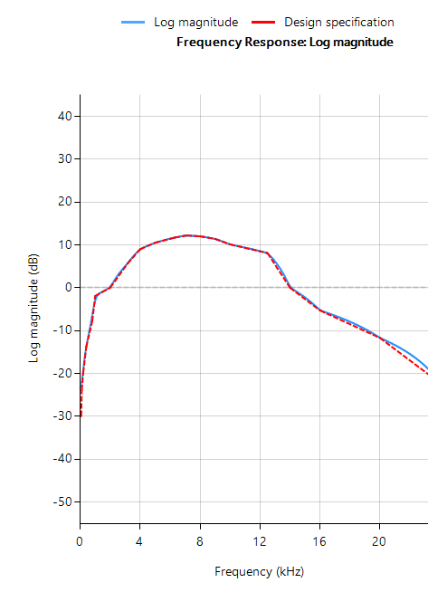
Frequency response of analog vs digital A-weighting filter for \(f_s=48kHz\). As seen, the digital equivalent magnitude response matches the ideal analog magnitude response very closely until \(6kHz\).
The ITU-R 486–4 weighting curve
Another weighting curve of interest is the ITU-R 486–4 weighting curve, developed by the BBC. Unlike the A-weighting filter, the ITU-R 468–4 curve describes subjective loudness for broadband stimuli. The main disadvantage of the A-weighting curve is that it underestimates the loudness judgement of real-world stimuli particularly in the frequency band from about 1–9 kHz.
Due to the precise definition of the 486–4 weighting curve, there is no analog transfer function available. Instead the standard provides a table of amplitudes and frequencies – see here. This specification may be directly entered into FilterScript’s firarb() function for designing a suitable FIR filter, as shown below:
ClearH1;  // clear primary filter from cascade
ShowH2DM;

interface L = {10,400,10,250}; // filter order

Main()

// ITU-R 468 Weighting
A={-29.9,-23.9,-19.8,-13.8,-7.8,-1.9,0,5.6,9,10.5,11.7,12.2,12,11.4,10.1,8.1,0,-5.3,-11.7,-22.2};
F={63,100,200,400,800,1e3,2e3,3.15e3,4e3,5e3,6.3e3,7.1e3,8e3,9e3,1e4,1.25e4,1.4e4,1.6e4,2e4};

A={-30,A};  //  specify arb response
F={0,F,fs/2};

Hd=firarb(L,A,F,"blackman","numeric");

Num=getnum(Hd);
Den={1};
Gain=getgain(Hd);
firarb() function for \(f_s=48kHz\)As seen, FilterScript provides the designer with a very powerful symbolic scripting language for designing weighting curve filters. The following discussion now focuses on deployment of the A-weighting filter to an Arm based processor via the tool’s automatic code generator. The concepts and steps demonstrated below are equally valid for FIR filters.
Automatic code generation to Arm processor cores via CMSIS-DSP
The ASN Filter Designer’s automatic code generation engine facilitates the export of a designed filter to Cortex-M Arm based processors via the CMSIS-DSP software framework.
The tool’s built-in analytics and help functions assist the designer in successfully configuring the design for deployment. Professional licence users may expedite the deployment by using the Arm deployment wizard that automates the steps described below.
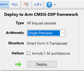
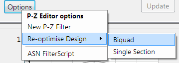
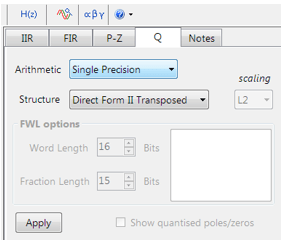
Before generating the code, the H2 filter (i.e. the filter designed in FilterScript) needs to be firstly re-optimised (transformed) to an H1 filter (main filter) structure for deployment. The options menu can be found under the P-Z tab in the main UI.
All floating point IIR filters designs must be based on Single Precision arithmetic and either a Direct Form I or Direct Form II Transposed filter structure. The Direct Form II Transposed structure is advocated for floating point implementation by virtue of its higher numerically accuracy.

Quantisation and filter structure settings can be found under the Q tab (as shown on the left). Setting Arithmetic to Single Precision and Structure to Direct Form II Transposed and clicking on the Apply button configures the IIR considered herein for the CMSIS-DSP software framework.
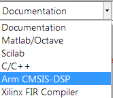
Select the Arm CMSIS-DSP framework from the selection box in the filter summary window:
The automatically generated C code based on the CMSIS-DSP framework for direct implementation on an Arm based Cortex-M processor is shown below:
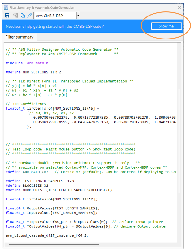
As seen, the ASN Filter Designer’s automatic code generator generates all initialisation code, scaling and data structures needed to implement the A-weighting filter IIR filter via Arm’s CMSIS-DSP library. A detailed help tutorial is available by clicking on the Show me button.

Author

In ECG signal processing, the Removal of 50/60Hz powerline interference from delicate information rich ECG biomedical waveforms is a challenging task! The challenge is further complicated by adjusting for the effects of EMG, such as a patient limb/torso movement or even breathing. A traditional approach adopted by many is to use a 2nd order IIR notch filter:
\(\displaystyle H(z)=\frac{1-2cosw_oz^{-1}+z^{-2}}{1-2rcosw_oz^{-1}+r^2z^{-2}}\)
where, \(w_o=\frac{2\pi f_o}{fs}\) controls the centre frequency, \(f_o\) of the notch, and \(r=1-\frac{\pi BW}{fs}\) controls the bandwidth (-3dB point) of the notch.
What’s the challenge?
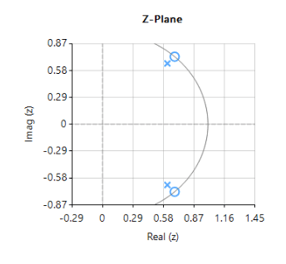
As seen above, \(H(z) \) is simple to implement, but the difficulty lies in finding an optimal value of \(r\), as a desirable sharp notch means that the poles are close to unit circle (see right).
In the presence of stationary interference, e.g. the patient is absolutely still and effects of breathing on the sensor data are minimal this may not be a problem.
However, when considering the effects of EMG on the captured waveform (a much more realistic situation), the IIR filter’s feedback (poles) causes ringing on the filtered waveform, as illustrated below:
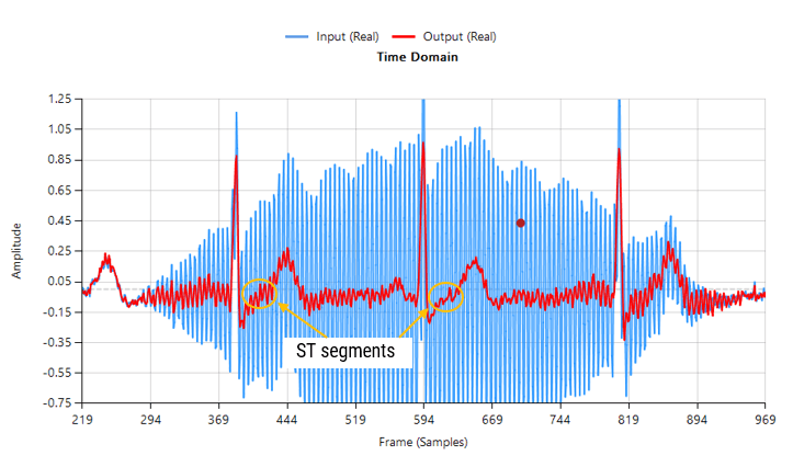
Contaminated ECG with non-stationary 50Hz powerline interference (IIR filtering)
As seen above, although a majority of the 50Hz powerline interference has been removed, there is still significant ringing around the main peaks (filtered output shown in red). This ringing is undesirable for many biomedical applications, as vital cardiac information such as the ST segment cannot be clearly analysed.
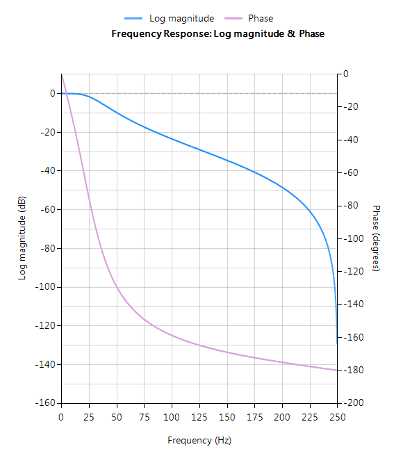
The frequency reponse of the IIR used to filter the above ECG data is shown below.
IIR notch filter frequency response
Analysing the plot it can be seen that the filter’s group delay (or average delay) is non-linear but almost zero in the passbands, which means no distortion. The group delay at 50Hz rises to 15 samples, which is the source of the ringing – where the closer to poles are to unit circle the greater the group delay.
ASN FilterScript offers designers the notch() function, which is a direct implemention of H(z), as shown below:
ClearH1;  // clear primary filter from cascade
ShowH2DM;   // show DM on chart

interface BW={0.1,10,.1,1};

Main()

F=50;
Hd=notch(F,BW,"symbolic");
Num = getnum(Hd); // define numerator coefficients
Den = getden(Hd); // define denominator coefficients
Gain = getgain(Hd); // define gain
Savitzky-Golay FIR filters
A solution to the aforementioned mentioned ringing as well as noise reduction can be achieved by virtue of a Savitzky-Golay lowpass smoothing filter. These filters are FIR filters, and thus have no feedback coefficients and no ringing!
Savitzky-Golay (polynomial) smoothing filters or least-squares smoothing filters are generalizations of the FIR average filter that can better preserve the high-frequency content of the desired signal, at the expense of not removing as much noise as an FIR average. The particular formulation of Savitzky-Golay filters preserves various moment orders better than other smoothing methods, which tend to preserve peak widths and heights better than Savitzky-Golay. As such, Savitzky-Golay filters are very suitable for biomedical data, such as ECG datasets.
Eliminating the 50Hz powerline component
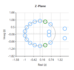
Designing an 18th order Savitzky-Golay filter with a 4th order polynomial fit (see the example code below), we obtain an FIR filter with a zero distribution as shown on the right. However, as we wish to eliminate the 50Hz component completely, the tool’s P-Z editor can be used to nudge a zero pair (shown in green) to exactly 50Hz.
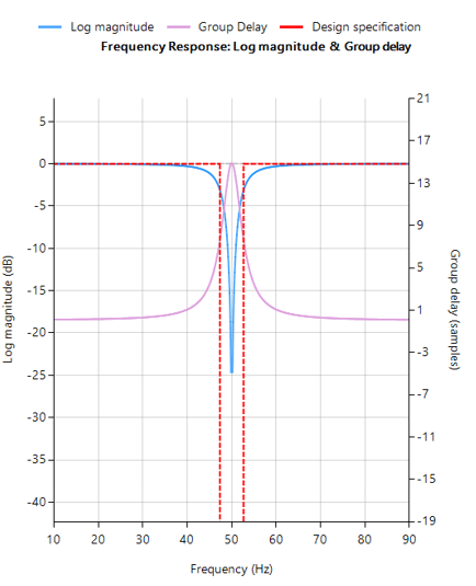
The resulting frequency response is shown below, where it can be seen that there is notch at exactly 50Hz, and the group delay of 9 samples (shown in purple) is constant across the frequency band.
FIR Savitzky-Golay filter frequency response
Passing the tainted ECG dataset through our tweaked Savitzky-Golay filter, and adjusting for the group delay we obtain:
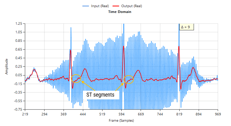
Contaminated ECG with non-stationary 50Hz powerline interference (FIR filtering)
As seen, there are no signs of ringing and the ST segments are now clearly visible for analysis. Notice also how the filter (shown in red) has reduced the measurement noise, emphasising the practicality of Savitzky-Golay filter’s for biomedical signal processing.
A Savitzky-Golay may be designed and optimised in ASN FilterScript via the savgolay() function, as follows:
ClearH1;  // clear primary filter from cascade

interface L = {2, 50,2,24};
interface P = {2, 10,1,4};

Main()

Hd=savgolay(L,P,"numeric");  // Design Savitzky-Golay lowpass
Num=getnum(Hd);
Den={1};
Gain=getgain(Hd);
Deployment
This filter may now be deployed to variety of domains via the tool’s automatic code generator, enabling rapid deployment in Matlab, Python and embedded Arm Cortex-M devices.
Author
In recent years, major microcontroller IC vendors such as: ST, NXP, TI, ADI, Atmel/Microchip, Cypress, Maxim to name but a few have based their modern 32-bit microcontrollers on Arm’s Cortex-M processor cores. This exciting trend means that algorithms traditionally undertaken in expensive DSPs (digital signal processors) can now be integrated into a powerful low-cost and power efficient microcontroller packed full of a rich assortment of connectivity and peripheral options.
For many IC vendors, the coupling of DSP functionality with the flexibility of a low power microcontroller, has allowed them to offer their customers a generation of so called 32-bit enhanced microcontrollers suitable for a variety of practical applications. More importantly, this marriage of technologies has also allowed designers working on price critical IoT applications to implement complex algorithmic concepts, while at the same time keeping the overall product cost low and still achieving excellent low power performance.
Upgrading legacy analog filters with the ASN Filter Designer
Analog filters have been around since the beginning of electronics, ranging from simple inductor-capacitor networks to more advanced active filters with op-amps. As such, there is a rich collection of tried and tested legacy filter designs for a broad range of sensor measurement applications.
ASN’s FilterScript symbolic math scripting language offers designers the ability to take an existing analog filter transfer function and transform it to digital with just a few lines of code. The ASN Filter Designer’s Arm automatic code generator analyses the designed digital filter and then automatically generates Arm CMSIS-DSP compliant C code suitable for direct implementation a Cortex-M based microcontroller.
Arm CMSIS-DSP software framework
The Arm CMSIS-DSP (Cortex Microcontroller Software Interface Standard) software framework is a rich collection of over sixty DSP functions (including various mathematical functions, such as sine and cosine; IIR/FIR filtering functions, complex math functions, and data types) developed by Arm that have been optimised for their range of Cortex-M processor cores. The framework makes extensive use of highly optimised SIMD (single instruction, multiple data) instructions, that perform multiple identical operations in a single cycle instruction. The SIMD instructions (if supported by the core) coupled together with other optimisations allow engineers to produce highly optimised signal processing applications for Cortex-M based micro-controllers quickly and simply.

Mathematically modelling an analog circuit
Consider the active pre-emphasis filter shown below. The pre-emphasis filter has found particular use in audio work, since it is necessary to amplify the higher frequencies of the speech spectrum, whilst leaving the lower frequencies unaffected. The R and C values shown are only indented for the example, more practical values will depend on the application.A powerful method of reproducing the magnitude and phases characteristics of the analog filter in a digital implementation, is to mathematically model the circuit. This circuit may be analysed using Kirchhoff’s law, since the sum of currents into the op-amp’s inverting input must be equal to zero for negative feedback to work correctly – this results in a transfer function with a negative gain.
Therefore, using Ohm’s law, i.e. \(I=\frac{V}{R}\),
\(\displaystyle\frac{X(s)}{R_3}=-\frac{U(s)}{C_1||R_2 + R_1}
\)
After some algebraic manipulation, it can be seen that an expression for the circuit’s closed loop gain may be expressed as,
\(\displaystyle\frac{X(s)}{U(s)}=-\frac{R_3}{R_1}\frac{\left(s+\frac{1}{R_2C_1}\right)}{\left(s+\frac{R_1+R_2}{R_1R_2C_1}\right)}
\)
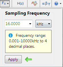
substituting the values shown in the circuit diagram into the developed transfer function, yields
\(\displaystyle H(s)=-10\left(\frac{s+1000}{s+11000}\right)
\)
What sampling rate do we need?
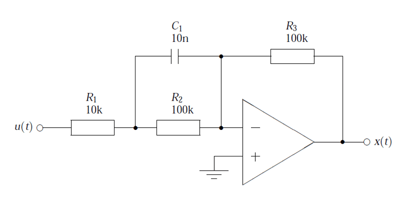
Analysing the cut-off frequencies in \(H(s)\), we see that the upper frequency is at \(11000 rad/sec\) or \(1.75kHz\). Therefore, setting the sampling rate to \(16kHz\) should be adequate for modelling the filter in the digital domain.
The sampling rate options are avaliabe in the main filter design UI (shown on the left).
ASN FilterScript
\(H(s)\) can be easily specified in FilterScript with the analogtf function, as follows:
Nb={1,1000};
Na={1,11000};

Ha=analogtf(Nb,Na,-10,"symbolic");
Notice how the negative gain may also be entered directly into function’s argument. The symbolic keyword generates a symbolic transfer function representation in the command window.
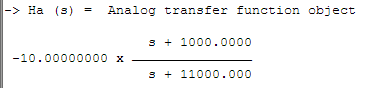
Applying the Bilinear z-transformation via the bilinear command with no pre-warping, i.e.
Hd=bilinear(Ha,0,"symbolic");
Notice how the bilinear command automatically scales numerator coefficients by -1, in order to account for the effect of the negative gain. The complete code is shown below:
Main()

Nb={1,1000};
Na={1,11000};

Ha=analogtf(Nb,Na,-10,"symbolic");
Hd=bilinear(Ha,0,"symbolic");

Num=getnum(Hd);
Den=getden(Hd);
Gain=getgain(Hd);
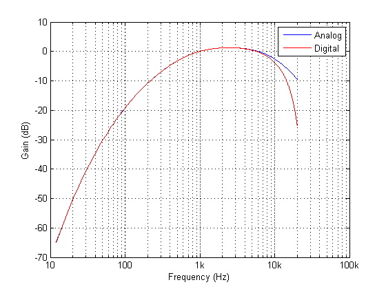
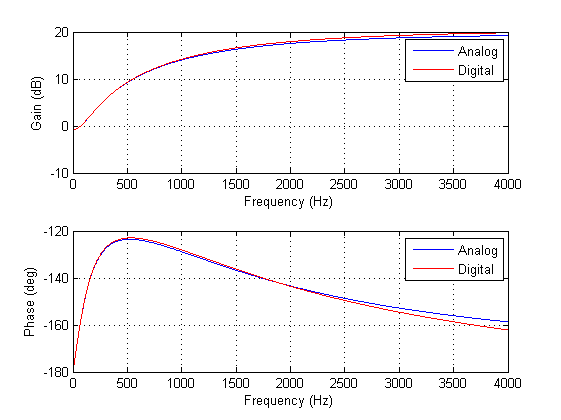
A comparison of the analog and discrete magnitude and phase spectra is shown below. Analysing the spectra, it can be seen that for a sampling rate of 16kHz the analog and digital filters are almost identical! This demonstrates the relative ease with which a designer can port their existing legacy analog designs into digital.
Automatic code generation to Arm Cortex-M processors
As mentioned at the beginning of this article, the ASN filter designer’s automatic code generation engine facilitates the export of a designed filter to Cortex-M Arm based processor cores via the CMSIS-DSP software framework. The tool’s built-in analytics and help functions assist the designer in successfully configuring the design for deployment.
Before generating the code, the H2 filter (i.e. the filter designed in FilterScript) needs to be firstly re-optimised (transformed) to an H1 filter (main filter) structure for deployment. The options menu can be found under the P-Z tab in the main UI.
All floating point IIR filters designs must be based on Single Precision arithmetic and either a Direct Form I or Direct Form II Transposed filter structure. The Direct Form II Transposed structure is advocated for floating point implementation by virtue of its higher numerically accuracy.
Quantisation and filter structure settings can be found under the Q tab (as shown on the left). Setting Arithmetic to Single Precision and Structure to Direct Form II Transposed and clicking on the Apply button configures the IIR considered herein for the CMSIS-DSP software framework.
Arm CMSIS-DSP application C code
Select the Arm CMSIS-DSP framework from the selection box in the filter summary window:
The automatically generated C code based on the CMSIS-DSP framework for direct implementation on an Arm based Cortex-M processor is shown below:
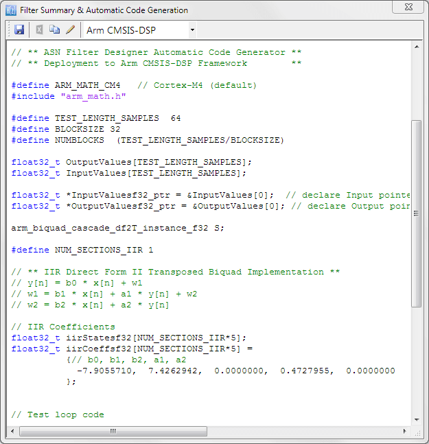
As seen, the automatic code generator generates all initialisation code, scaling and data structures needed to implement the IIR via the CMSIS-DSP library. This code may be directly used in any Cortex-M based development project – a complete Keil MDK example is available on Arm/Keil’s website. Notice that the tool’s code generator produces code for the Cortex-M4 core as default, please refer to the table below for the #define definition required for all supported cores.
ARM_MATH_CM0 | Cortex-M0 core. | ARM_MATH_CM4 | Cortex-M4 core. |
ARM_MATH_CM0PLUS | Cortex-M0+ core. | ARM_MATH_CM7 | Cortex-M7 core. |
ARM_MATH_CM3 | Cortex-M3 core. | ||
ARM_MATH_ARMV8MBL | ARMv8M Baseline target (Cortex-M23 core). | ||
ARM_MATH_ARMV8MML | ARMv8M Mainline target (Cortex-M33 core). |
The main test loop code (not shown) centres around the arm_biquad_cascade_df2T_f32() function, which performs the filtering operation on a block of input data.
What have we learned?
The ASN Filter Designer provides engineers with everything they need in order to port legacy analog filter designs to a variety of Cortex-M processor cores.
The FilterScript symbolic math scripting language offers designers the ability to take an existing analog filter transfer function and transform it to digital (via the Bilinear z-transform or matched z-transform) with just a few lines of code.
The Arm automatic code generator analyses the designed digital filter and then automatically generates Arm CMSIS-DSP compliant C code suitable for direct implementation on a Cortex-M based microcontroller.
Extra resources
- Step by step video tutorial of designing an IIR and deploying it to Keil MDK uVision.
- Implementing Biquad IIR filters with the ASN Filter Designer and the Arm CMSIS-DSP software framework (ASN-AN025)
- Keil MDK uVision example IIR filter project
- Step by step instruction video of this tutorial Arm Webinar (requires registration)
Upgrading legacy designs based on analog filters
Analog filters have been around since the beginning of electronics, ranging from simple inductor-capacitor networks to more advanced active filters with op-amps. As such, there is a rich collection of tried and tested legacy filter designs for a broad range of sensor measurement applications. However, with the performance requirements of modern IoT (Internet of Things) sensor measurement applications and lower product costs, digital filters integrated into the microcontroller’s application code are becoming the norm, but how can we get the best of both worlds?
Rather than re-inventing the wheel, product designers can take an existing analog filter transfer function, transform it to digital (via a transform) and implement it as digital filter in a microcontroller or DSP (digital signal processor). Although analog-to-digital transforms have been around for decades, the availability of DSP design tooling for tweaking the ‘transformed digital filter’ has been somewhat limited, hindering the design and validation process.
A 2nd order analog lowpass filter is shown below, and in its simplest form, only 5 components are required to build the filter, which sounds easy. Right?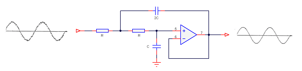
The pros
The most obvious advantage is that analog filters have an excellent resolution, as there are no ‘number of bits’ to consider. Analog filters have good EMC (electromagnetic compatibility) properties as there is no clock generating noise. There are no effects of aliasing, which is certainly true for the simpler op-amps, which don’t have any fancy chopping or auto-calibration circuitry built into them, and analog designs can be cheap which is great for cost sensitive applications.
Sound great, but what’s the bad news?
Analog filters have several significant disadvantages that affect filter performance, such as component aging, temperature drift and component tolerance. Also, good performance requires good analog design skills and good PCB (printed circuit board) layout, which is hard to find in the contemporary skills market.
These disadvantages make digital filters much more attractive for modern applications, that require high repeatability of characteristics. Looking at an example, let’s say that you want to manufacture 1000 measurement modules after optimising your filter design. With a digital solution you can be sure that the performance of your filter will be identical in all modules. This is certainly not the case with analog, as component tolerance, component aging and temperature drift mean that each module’s filter will have its own characteristics. Also, an analog filter’s frequency response remains fixed, i.e. a Butterworth filter will always be a Butterworth filter – any changes the frequency response would require physically changing components on the PCB – not ideal!
Digital filters are adaptive and flexible, we can design and implement a filter with any frequency response that we want, deploy it and then update the filter coefficients without changing anything on the PCB! It’s also easy to design digital filters with linear phase and at very low sampling frequencies – two things that are tricky with analog.
Laplace to discrete/digital transforms
The three methods discussed herein essentially involve transforming a Laplace (analog) transfer function, \(H(s)\) into a discrete transfer function, \(H(z)\) such that a tried and tested analog filter that is already used in a design may be implemented on a microcontroller or DSP.
A selection of some useful Laplace to z-transforms are given in table below:
\(
\begin{array}{ccc}\hline
H(s) &\longleftrightarrow & H(z) \\ \hline
1 &\longleftrightarrow & 1 \\
\frac{\displaystyle1}{\displaystyle s}
&\longleftrightarrow& \frac{\displaystyle 1}{\displaystyle 1-z^{\scriptstyle -1}}\\
\frac{\displaystyle 1}{\displaystyle s^{\scriptstyle 2}} &\longleftrightarrow& \frac{\displaystyle
Tz^{\scriptstyle-1}}{\displaystyle (1-z^{\scriptstyle -1})^2}\\
\frac{\displaystyle 1}{\displaystyle s+a}
&\longleftrightarrow&
\frac{\displaystyle 1}{\displaystyle 1-e^{-aT}z^{-1}}\\
\frac{\displaystyle 1}{\displaystyle (s+a)^2}
&\longleftrightarrow& \frac{\displaystyle z^{-1}(1-e^{-aT})}{\displaystyle a(1-z^{-1})(1-e^{-aT}z^{-1})}\\\hline
\end{array}
\)
A table of useful Laplace and z-transforms
The Bilinear z-transform (BZT)
The Bilinear z-transform (BZT), simply converts an analog transfer function, \(H(s)\) into a discrete transfer function, \(H(z)\) by replacing all \(s\) terms with the following:
\(\displaystyle
s=\frac{2}{T}\frac{1-z^{-1}}{1+z^{-1}} \label{bzt}\)
where, \(T\) is the discrete system’s sampling period. However, substituting \(s=j\Omega\) and \(z=e^{jwT}\) into the BZT equation and simplifying, notice that there is actually a non-linear relationship between the analog, \(\Omega\) and discrete, \(w\) frequencies. This relationship is shown below, and is due to the nonlinearity of the arctangent function.
\(\displaystyle\omega=2\tan^{-1}\left(\frac{\Omega T}{2}\right)\label{bzt_warp_def1}\)
Analysing the equation, it can be seen that the equally spaced analog frequencies in the range \( -\infty\lt\Omega\lt\infty\) are nonlinearly compressed in the frequency range \( -\pi\lt w\lt\pi\) in the discrete domain. This relationship is referred to as frequency warping, and may be compensated for by pre-warping the analog frequencies by:
\(\displaystyle
\Omega_c=\frac{2}{T}\tan\left(\frac{\Omega_d T}{2}\right)
\label{bzt_warp_def2}
\)
where, \(\displaystyle\Omega_c\) is the compensated or pre-warped analog frequency, and \(\displaystyle\Omega_d\) is the desired analog frequency.
The ASN FilterScript command \(\texttt{bilinear}\) may be used convert a Laplace transfer function into its discrete equivalent using the BZT transform. An example is given below.
The Impulse Invariant Transform
The second transform, is referred to as the impulse invariant transform (IIT), since the poles of the Laplace transfer function are converted into their discrete equivalents, such that the discrete impulse response, \(h(n)\) is identical to a regularly sampled representation of the analog impulse response (i.e., \(h(n)=h(nT)\), where \(T\) is the sampling rate, and \(t=nT\)). The IIT is a much more tedious transformation technique than the BZT, since the Laplace transfer function must be firstly expanded using partial fractions before applying the transform.
The transformation technique is defined below:
\(\displaystyle
\frac{K}{s+a} \quad\longrightarrow\quad
\frac{K}{1-e^{-aT}z^{-1}} \label{iit_def}
\)
This method suffers from several constraints, since it does not allow for the transformation of zeros or individual constant terms (once expanded), and must have a high sampling rate in order to overcome the effects of spectral aliasing. Indeed, the effects of aliasing hinder this method considerably, such that the method should only be used when the requirement is to match the analog transfer function’s impulse response, since the resulting discrete model may have a different magnitude and phase spectrum (frequency response) to that of the original analog system. Consequently, the impulse invariant method is unsuitable for modelling highpass filters, and is therefore limited to the modelling of lowpass or bandpass type filters.
Due to the aforementioned limitations of the IIT method, it is currently not supported in ASN Filterscript.
The Matched-z transformation
Another analog to discrete modelling technique is the matched-z transformation. As the name suggests, the transform converts the poles and zeros from the analog transfer function directly into poles and zeros in the z-plane. The transformation is described below, where \(T\) is the sampling rate.
\(\displaystyle
\frac{\prod\limits_{k=1}^q(s+b_k)}{\prod\limits_{k=1}^p(s+a_k)}
\quad\longrightarrow\quad
\frac{\prod\limits_{k=1}^q(1-e^{-b_kT}z^{-1})}{\prod\limits_{k=1}^p(1-e^{-a_kT}z^{-1})}
\label{matchedz_def}
\)
Analysing the transform equation, it can be seen that the transformed z-plane poles will be identical to the poles obtained with the impulse invariant method. However, notice that the positions of the zeros will be different, since the impulse invariant method cannot transform them.
The ASN Filterscript command \(\texttt{mztrans}\) is available for this method.
A detailed example
In order to demonstrate the ease of transforming analog filters into their discrete/digital equivalents using the analog to discrete transforms, an example of modelling with the BZT will now follow for a 2nd order lowpass analog filter.
A generalised 2nd order lowpass analog filter is given by:
\(\displaystyle
H(s)=\frac{w_c^2}{s^2+2\zeta w_c s + w_c^2}
\)
where, \(w_c=2\pi f_c\) is the cut-off frequency and \(\zeta\) sets the damping of the filter, where a \(\zeta=1/\sqrt{2}\) is said to be critically damped or equal to -3dB at \(w_c\). Many analog engineers choose to specify a quality factor, \(Q = \displaystyle\frac{1}{2\zeta}\) or peaking factor for their designs. Substituting \(Q\) into \(H(s)\), we obtain:
\(\displaystyle
H(s)=\frac{w_c^2}{s^2+ \displaystyle{\frac{w_c}{Q}s} + w_c^2}
\)
Analysing, \(H(s)\) notice that \(Q=1/\sqrt{2} = 0.707\) also results in a critically damped response. Various values of \(Q\) are shown below, and as seen when \(Q>1/\sqrt{2}\) peaking occurs.
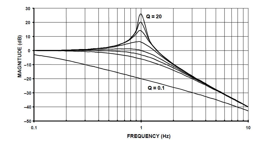
2nd order lowpass filter prototype magnitude spectrum for various value of Q:
notice that when \(Q>1/\sqrt{2}\) peaking occurs.
Before applying the BZT in ASN FilterScript, the analog transfer function must be specified in an analog filter object. The following code sets up an analog filter object for the 2nd order lowpass prototype considered herein:
Main()

wc=2*pi*fc;
Nb={0,0,wc^2};
Na={1,wc/Q,wc^2};

Ha=analogtf(Nb,Na,1,"symbolic"); // make analog filter object
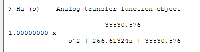
The \(\texttt{symbolic}\) keyword generates a symbolic transfer function representation in the command window. For a sampling rate of \(f_s=500Hz\) and \(f_c=30Hz\) and \(Q=0.707\), we obtain:
Applying the BZT via the \(\texttt{bilinear}\) command without prewarping,
Hd=bilinear(Ha,0,"symbolic");
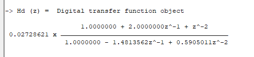
The complete frequency response of the transformed digital filter is shown below, where it can be seen that the at \(30Hz\) the magnitude is \(-3dB\) and the phase is \( -90^{\circ}\), which is as expected. Notice also how the filter’s magnitude roll-off is affected by the double zero pair at Nyquist (see the z-plane chart below), leading to differences from its analog cousin. 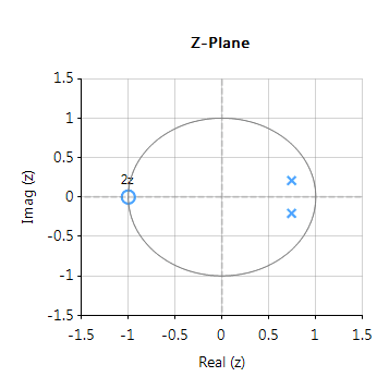
The pole-zero positions may be tweaked within ASN Filterscript or via the ASN Filter Designer’s interactive pole-zero z-plane plot editor by just using the mouse!
Implementation
The complete code for transforming a generalised 2nd order analog lowpass filter prototype into its digital equivalent using the BZT via ASN FilterScript is given below:
ClearH1;  // clear primary filter from cascade
interface Q = {0.1,10,0.02,0.707};
interface fc = {10,200,10,40};

Main()

wc=2*pi*fc;
Nb={0,0,wc^2};
Na={1,wc/Q,wc^2};

Ha=analogtf(Nb,Na,1,"symbolic"); // make analog filter object
Hd=bilinear(Ha,0,"symbolic"); // transform Ha via BZT into digital object, Hd

Num=getnum(Hd);
Den=getden(Hd);
Gain=getgain(Hd);
Author
All-pass filters
All-pass filters provide a simple way of altering/improving the phase response of an IIR without affecting its magnitude response. As such, they are commonly referred to as phase equalisers and have found particular use in digital audio applications. In its simplest form, a filter can be constructed from a first order transfer function, i.e., \( A(z)=\Large{\frac{r+z^{-1}}{1+r z^{-1}}} \, \, \normalsize{; r<1} \) Analysing \(\small A(z)\), notice that the pole and zero lie on the real z-plane axis and that the pole at radius \(\small r\) has a zero at radius \(\small 1/r\), such that the poles and zeros are reciprocals of another. This property is key to the all-pass filter concept, as we will now see by expanding the concept further to a second order all-pass filter: \( A(z)=\Large\frac{r^2-2rcos \left( \frac{2\pi f_c}{fs}\right) z^{-1}+z^{-2}}{1-2rcos \left( \frac{2\pi f_c}{fs}\right)z^{-1}+r^2 z^{-2}} \) Where, \(\small f_c\) is the centre frequency, \(\small r\) is radius of the poles and An All-pass filter may be implemented in ASN FilterScript as follows: For a detailed discussion on IIR filter phase equalisation, and the ASN Filter designer’s APF (all-pass filter) design tool, please refer to the following article. 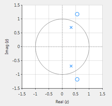 \(\small f_s\) is the sampling frequency. Notice how the numerator and denominator coefficients are arranged as a mirror image pair of one another. The mirror image property is what gives the all-pass filter its desirable property, namely allowing the designer to alter the phase response while keeping the magnitude response constant or flat over the complete frequency spectrum.
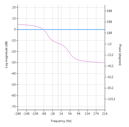 Frequency response of all-pass filter:
Notice the constant magnitude spectrum (shown in blue). Implementation
ClearH1;  // clear primary filter from cascade

interface radius = {0,2,0.01,0.5};   // radius value
interface fc = {0,fs/2,1,fs/10};     // frequency value

Main()
Num = {radius^2,-2*radius*cos(Twopi*fc/fs),1};
Den = reverse(Num); // mirror image of Num
Gain = 1;
Author
A Peaking or Bell filter is a type of audio equalisation filter that boosts or attenuates the magnitude of a specified set of frequencies around a centre frequency in order to perform magnitude equalisation. As seen in the plot in the below, the filter gets its name from the shape of the its magnitude spectrum (blue line) which resembles a Bell curve.
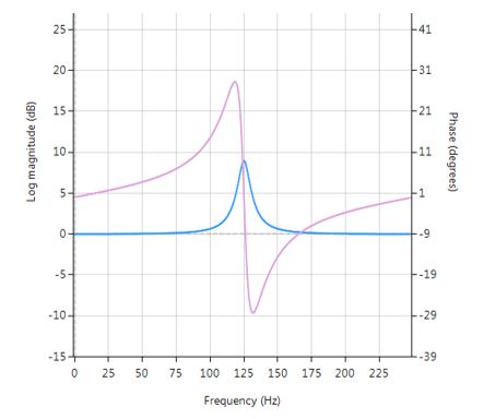
Frequency response (magnitude shown in blue, phase shown in purple) of a 2nd order Bell filter peaking at 125Hz.
All-pass filters
Central to the Bell filter is the so called All-pass filter. All-pass filters provide a simple way of altering/improving the phase response of an IIR without affecting its magnitude response. As such, they are commonly referred to as phase equalisers and have found particular use in digital audio applications.
A second order all-pass filter is defined as:
\( A(z)=\Large\frac{r^2-2rcos \left( \frac{2\pi f_c}{fs}\right) z^{-1}+z^{-2}}{1-2rcos \left( \frac{2\pi f_c}{fs}\right)z^{-1}+r^2 z^{-2}} \)
Notice how the numerator and denominator coefficients are arranged as a mirror image pair of one another. The mirror image property is what gives the all-pass filter its desirable property, namely allowing the designer to alter the phase response while keeping the magnitude response constant or flat over the complete frequency spectrum.
A Bell filter can be constructed from the \(A(z)\) filter by the following transfer function:
\(H(z)=\Large\frac{(1+K)+A(z)(1-K)}{2}\)
After some algebraic simplication, we obtain the transfer function for the Peaking or Bell filter as:
\(H(z)=\Large{\frac{1}{2}}\left[\normalsize{(1+K)} + \underbrace{\Large\frac{k_2 + k_1(1+k_2)z^{-1}+z^{-2}}{1+k_1(1+k_2)z^{-1}+k_2 z^{-2}}}_{all-pass filter}\normalsize{(1-K)} \right] \)
- \(K\) is used to set the gain and sign of the peak
- \(k_1\) sets the peak centre frequency
- \(k_2\) sets the bandwidth of the peak
Implementation
A Bell filter may easily be implemented in ASN FilterScript as follows:
ClearH1;  // clear primary filter from cascade
interface BW = {0,2,0.1,0.5}; // filter bandwidth
interface fc = {0, fs/2,fs/100,fs/4}; // peak/notch centre frequency
interface K = {0,3,0.1,0.5}; // gain/sign

Main()

k1=-cos(2*pi*fc/fs);
k2=(1-tan(BW/2))/(1+tan(BW/2));

Pz = {1,k1*(1+k2),k2}; // define denominator coefficients
Qz = {k2,k1*(1+k2),1}; // define numerator coefficients
Num = (Pz*(1+K) + Qz*(1-K))/2;
Den = Pz;
Gain = 1;
This code may now be used to design a suitable Bell filter, where the exact values of \(K, f_c\) and \(BW\) may be easily found by tweaking the interface variables and seeing the results in real-time, as described below.
Designing the filter on the fly
Central to the interactivity of the FilterScript IDE (integrated development environment) are the so called interface variables. An interface variable is simply stated: a scalar input variable that can be used modify a symbolic expression without having to re-compile the code – allowing designers to design on the fly and quickly reach an optimal solution.
As seen in the code example above, interface variables must be defined in the initialisation section of the code, and may contain constants (such as, fs and pi) and simple mathematical operators, such as multiply * and / divide. Where, adding functions to an interface variable is not supported.
An interface variable is defined as vector expression:
interface name = {minimum, maximum, step_size, default_value};
Where, all entries must be real scalars values. Vectors and complex values will not compile.
Real-time updates
All interface variables are modified via the interface variable controller GUI. After compiling the code, use the interface variable controller to tweak the interface variables values and see the effects on the transfer function. If testing on live audio, you may stream a loaded audio file and adjust the interface variables in real-time in order to hear the effects of the new settings.