A digital filter is a mathematical algorithm that operates on a digital dataset (e.g. sensor data) in order extract information of interest and remove any unwanted information. Applications of this type of technology, include removing glitches from sensor data or even cleaning up noise on a measured signal for easier data analysis. But how do we choose the best type of digital filter for our application? And what are the differences between an IIR filter and an FIR filter?
Digital filters are divided into the following two categories:
- Infinite impulse response (IIR)
- Finite impulse response (FIR)
As the names suggest, each type of filter is categorised by the length of its impulse response. However, before beginning with a detailed mathematical analysis, it is prudent to appreciate the differences in performance and characteristics of each type of filter.
Example
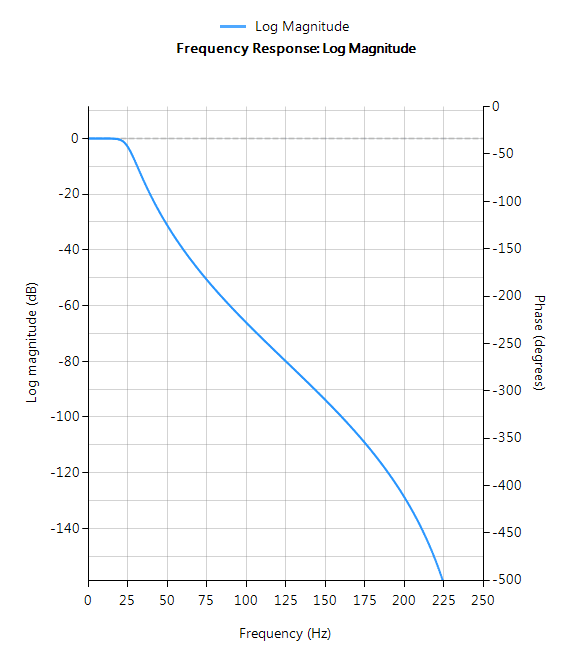
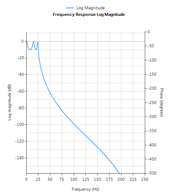
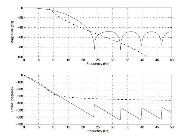
In order to illustrate the differences between an IIR and FIR, the frequency response of a 14th order FIR (solid line), and a 4th order Chebyshev Type I IIR (dashed line) is shown below in Figure 1. Notice that although the magnitude spectra have a similar degree of attenuation, the phase spectrum of the IIR filter is non-linear in the passband (\(\small 0\rightarrow7.5Hz\)), and becomes very non-linear at the cut-off frequency, \(\small f_c=7.5Hz\). Also notice that the FIR requires a higher number of coefficients (15 vs the IIR’s 10) to match the attenuation characteristics of the IIR.
These are just some of the differences between the two types of filters. A detailed summary of the main advantages and disadvantages of each type of filter will now follow.
IIR filters
IIR (infinite impulse response) filters are generally chosen for applications where linear phase is not too important and memory is limited. They have been widely deployed in audio equalisation, biomedical sensor signal processing, IoT/IIoT smart sensors and high-speed telecommunication/RF applications.
Advantages
- Low implementation cost: requires less coefficients and memory than FIR filters in order to satisfy a similar set of specifications, i.e., cut-off frequency and stopband attenuation.
- Low latency: suitable for real-time control and very high-speed RF applications by virtue of the low number of coefficients.
- Analog equivalent: May be used for mimicking the characteristics of analog filters using s-z plane mapping transforms.
Disadvantages
- Non-linear phase characteristics: The phase charactersitics of an IIR filter are generally nonlinear, especially near the cut-off frequencies. All-pass equalisation filters can be used in order to improve the passband phase characteristics.
- More detailed analysis: Requires more scaling and numeric overflow analysis when implemented in fixed point. The Direct form II filter structure is especially sensitive to the effects of quantisation, and requires special care during the design phase.
- Numerical stability: Less numerically stable than their FIR (finite impulse response) counterparts, due to the feedback paths.
FIR filters
FIR (finite impulse response) filters are generally chosen for applications where linear phase is important and a decent amount of memory and computational performance are available. They have a widely deployed in audio and biomedical signal enhancement applications. Their all-zero structure (discussed below) ensures that they never become unstable for any type of input signal, which gives them a distinct advantage over the IIR.
Advantages
- Linear phase: FIRs can be easily designed to have linear phase. This means that no phase distortion is introduced into the signal to be filtered, as all frequencies are shifted in time by the same amount – thus maintaining their relative harmonic relationships (i.e. constant group and phase delay). This is certainly not case with IIR filters, that have a non-linear phase characteristic.
- Stability: As FIRs do not use previous output values to compute their present output, i.e. they have no feedback, they can never become unstable for any type of input signal, which is gives them a distinct advantage over IIR filters.
- Arbitrary frequency response: The Parks-McClellan and ASN FilterScript’s firarb() function allow for the design of an FIR with an arbitrary magnitude response. This means that an FIR can be customised more easily than an IIR.
- Fixed point performance: the effects of quantisation are less severe than that of an IIR.
Disadvantages
- High computational and memory requirement: FIRs usually require many more coefficients for achieving a sharp cut-off than their IIR counterparts. The consequence of this is that they require much more memory and significantly a higher amount of MAC (multiple and accumulate) operations. However, modern microcontroller architectures based on the Arm’s Cortex-M cores now include DSP hardware support via SIMD (signal instruction, multiple data) that expedite the filtering operation significantly.
- Higher latency: the higher number of coefficients, means that in general a linear phase FIR is less suitable than an IIR for fast high throughput applications. This becomes problematic for real-time closed-loop control applications, where a linear phase FIR filter may have too much group delay to achieve loop stability.
- Minimum phase filters: A solution to ovecome the inherent N/2 latency (group delay) in a linear filter is to use a so-called minimum phase filter, whereby any zeros outside of the unit circle are moved to their conjugate reciprocal locations inside the unit circle. The result of the zero flipping operation is that the magnitude spectrum will be identical to the original filter, and the phase will be nonlinear, but most importantly the latency will be reduced from N/2 to something much smaller (although non-constant), making it suitable for real-time control applications.
For applications where phase is less important, this may sound ideal, but the difficulty arises in the numerical accuracy of the root-finding algorithm when dealing with large polynomials. Therefore, orders of 50 or 60 should be considered a maximum when using this approach. Although other methods do exist (e.g. the Complex Cepstrum), transforming higher-order linear phase FIRs to their minimum phase cousins remains a challenging task. - No analog equivalent: using the Bilinear, matched z-transform (s-z mapping), an analog filter can be easily be transformed into an equivalent IIR filter. However, this is not possible for an FIR as it has no analog equivalent.
Mathematical definitions
As discussed in the introduction, the name IIR and FIR originate from the mathematical definitions of each type of filter, i.e. an IIR filter is categorised by its theoretically infinite impulse response,
y(n)=\sum_{k=0}^{\infty}h(k)x(n-k)
\)
and an FIR categorised by its finite impulse response,
y(n)=\sum_{k=0}^{N-1}h(k)x(n-k)
\)
We will now analyse the mathematical properties of each type of filter in turn.
IIR definition
As seen above, an IIR filter is categorised by its theoretically infinite impulse response,
\(\displaystyle y(n)=\sum_{k=0}^{\infty}h(k)x(n-k) \)
Practically speaking, it is not possible to compute the output of an IIR using this equation. Therefore, the equation may be re-written in terms of a finite number of poles \(\small p\) and zeros \(\small q\), as defined by the linear constant coefficient difference equation given by:
y(n)=\sum_{k=0}^{q}b_k x(n-k)-\sum_{k=1}^{p}a_ky(n-k)
\)
where, \(\small a_k\) and \(\small b_k\) are the filter’s denominator and numerator polynomial coefficients, who’s roots are equal to the filter’s poles and zeros respectively. Thus, a relationship between the difference equation and the z-transform (transfer function) may therefore be defined by using the z-transform delay property such that,
\sum_{k=0}^{q}b_kx(n-k)-\sum_{k=1}^{p}a_ky(n-k)\quad\stackrel{\displaystyle\mathcal{Z}}{\longleftrightarrow}\quad\frac{\sum\limits_{k=0}^q b_kz^{-k}}{1+\sum\limits_{k=1}^p a_kz^{-k}}
\)
As seen, the transfer function is a frequency domain representation of the filter. Notice also that the poles act on the output data, and the zeros on the input data. Since the poles act on the output data, and affect stability, it is essential that their radii remain inside the unit circle (i.e. <1) for BIBO (bounded input, bounded output) stability. The radii of the zeros are less critical, as they do not affect filter stability. This is the primary reason why all-zero FIR (finite impulse response) filters are always stable.
BIBO stability
A linear time invariant (LTI) system (such as a digital filter) is said to be bounded input, bounded output stable, or BIBO stable, if every bounded input gives rise to a bounded output, as
\(\displaystyle \sum_{k=0}^{\infty}\left|h(k)\right|<\infty \)
Where, \(\small h(k)\) is the LTI system’s impulse response. Analyzing this equation, it should be clear that the BIBO stability criterion will only be satisfied if the system’s poles lie inside the unit circle, since the system’s ROC (region of convergence) must include the unit circle. Consequently, it is sufficient to say that a bounded input signal will always produce a bounded output signal if all the poles lie inside the unit circle.
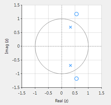
The zeros on the other hand, are not constrained by this requirement, and as a consequence may lie anywhere on z-plane, since they do not directly affect system stability. Therefore, a system stability analysis may be undertaken by firstly calculating the roots of the transfer function (i.e., roots of the numerator and denominator polynomials) and then plotting the corresponding poles and zeros upon the z-plane.
An interesting situation arises if any poles lie on the unit circle, since the system is said to be marginally stable, as it is neither stable or unstable. Although marginally stable systems are not BIBO stable, they have been exploited by digital oscillator designers, since their impulse response provides a simple method of generating sine waves, which have proved to be invaluable in the field of telecommunications.
Biquad IIR filters
The IIR filter implementation discussed herein is said to be biquad, since it has two poles and two zeros as illustrated below in Figure 2. The biquad implementation is particularly useful for fixed point implementations, as the effects of quantization and numerical stability are minimised. However, the overall success of any biquad implementation is dependent upon the available number precision, which must be sufficient enough in order to ensure that the quantised poles are always inside the unit circle.
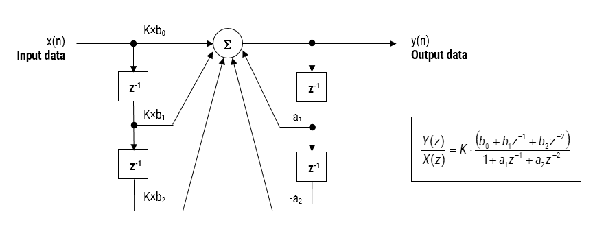
Figure 2: Direct Form I (biquad) IIR filter realization and transfer function.
Analysing Figure 2, it can be seen that the biquad structure is actually comprised of two feedback paths (scaled by \(\small a_1\) and \(\small a_2\)), three feed forward paths (scaled by \(\small b_0, b_1\) and \(\small b_2\)) and a section gain, \(\small K\). Thus, the filtering operation of Figure 1 can be summarised by the following simple recursive equation:
\(\displaystyle y(n)=K\times\Big[b_0 x(n) + b_1 x(n-1) + b_2 x(n-2)\Big] – a_1 y(n-1)-a_2 y(n-2)\)
Analysing the equation, notice that the biquad implementation only requires four additions (requiring only one accumulator) and five multiplications, which can be easily accommodated on any Cortex-M microcontroller. The section gain, \(\small K\) may also be pre-multiplied with the forward path coefficients before implementation.
A collection of Biquad filters is referred to as a Biquad Cascade, as illustrated below.
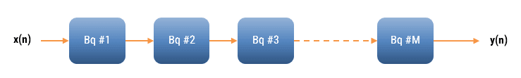
The ASN Filter Designer can design and implement a cascade of up to 50 biquads (Professional edition only).
Floating point implementation
When implementing a filter in floating point (i.e. using double or single precision arithmetic) Direct Form II structures are considered to be a better choice than the Direct Form I structure. The Direct Form II Transposed structure is considered the most numerically accurate for floating point implementation, as the undesirable effects of numerical swamping are minimised as seen by analysing the difference equations.
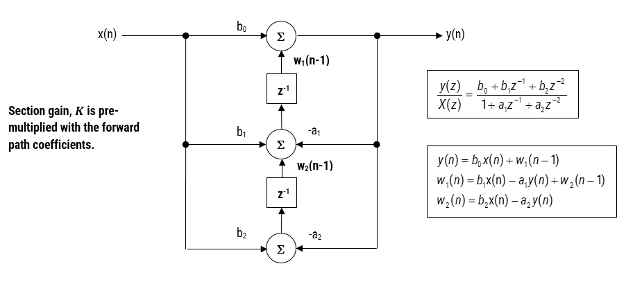
Figure 3 – Direct Form II Transposed strucutre, transfer function and difference equations
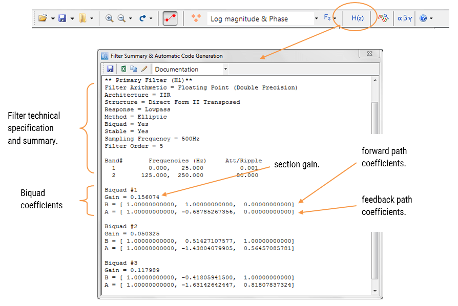
The filter summary (shown in Figure 4) provides the designer with a detailed overview of the designed filter, including a detailed summary of the technical specifications and the filter coefficients, which presents a quick and simple route to documenting your design.

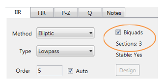
The ASN Filter Designer supports the design and implementation of both single section and Biquad (default setting) IIR filters.
FIR definition
Returning the IIR’s linear constant coefficient difference equation, i.e.
y(n)=\sum_{k=0}^{q}b_kx(n-k)-\sum_{k=1}^{p}a_ky(n-k)
\)
Notice that when we set the \(\small a_k\) coefficients (i.e. the feedback) to zero, the definition reduces to our original the FIR filter definition, meaning that the FIR computation is just based on past and present inputs values, namely:
y(n)=\sum_{k=0}^{q}b_kx(n-k)
\)
Implementation
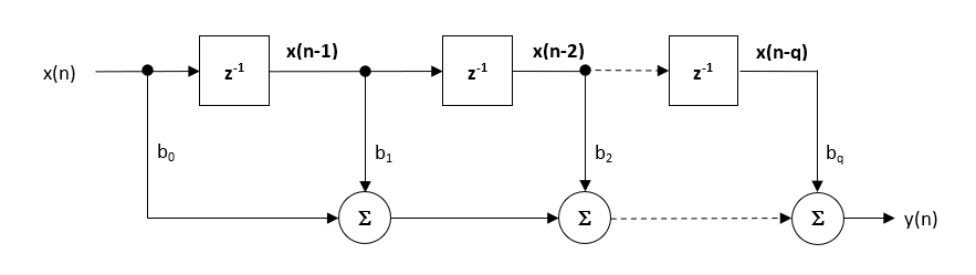
Although several practical implementations for FIRs exist, the direct form structure and its transposed cousin are perhaps the most commonly used, and as such, all designed filter coefficients are intended for implementation in a Direct form structure.
The Direct form structure and associated difference equation are shown below. The Direct Form is advocated for fixed point implementation by virtue of the single accumulator concept.
\(\displaystyle y(n) = b_0x(n) + b_1x(n-1) + b_2x(n-2) + …. +b_qx(n-q) \)
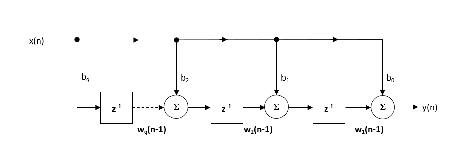
The recommended (default) structure within the ASN Filter Designer is the Direct Form Transposed structure, as this offers superior numerical accuracy when using floating point arithmetic. This can be readily seen by analysing the difference equations below (used for implementation), as the undesirable effects of numerical swamping are minimised, since floating point addition is performed on numbers of similar magnitude.
\(\displaystyle \begin{eqnarray}y(n) & = &b_0x(n) &+& w_1(n-1) \\ w_1(n)&=&b_1x(n) &+& w_2(n-1) \\ w_2(n)&=&b_2x(n) &+& w_3(n-1) \\ \vdots\quad &=& \quad\vdots &+&\quad\vdots \\ w_q(n)&=&b_qx(n) \end{eqnarray}\)
What have we learned?
Digital filters are divided into the following two categories:
- Infinite impulse response (IIR)
- Finite impulse response (FIR)
IIR (infinite impulse response) filters are generally chosen for applications where linear phase is not too important and memory is limited. They have been widely deployed in audio equalisation, biomedical sensor signal processing, IoT/IIoT smart sensors and high-speed telecommunication/RF applications.
FIR (finite impulse response) filters are generally chosen for applications where linear phase is important and a decent amount of memory and computational performance are available. They have a widely deployed in audio and biomedical signal enhancement applications.
ASN Filter Designer provides engineers with everything they need to design, experiment and deploy complex IIR and FIR digital filters for a variety of sensor measurement applications. These advantages coupled with automatic C code generation functionality allow engineers to design, validate and then deploy their designs to an Arm Cortex-M processor within hours rather than more traditional routes that could take days.