computationally-efficient-moving-average-filter

As discussed in a previous article, the moving average (MA) filter is perhaps one of the most widely used digital filters due to its conceptual simplicity and ease of implementation. The realisation diagram shown below, illustrates that an MA filter can be implemented as a simple FIR filter, just requiring additions and a delay line.

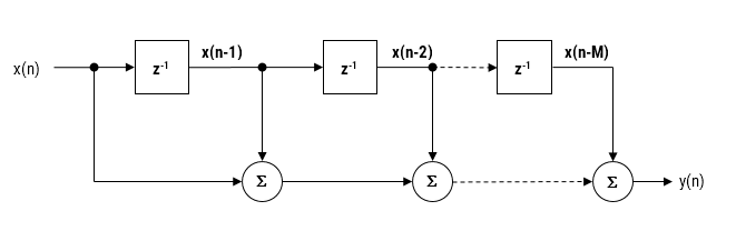
moving average filter, an MA filter can be implemented as a simple FIR filter, just requiring additions and a delay line. moving average FIR filter

Modelling the above, we see that a moving average filter of length \(\small\textstyle L\) for an input signal \(\small\textstyle x(n)\) may be defined as follows:

\( y(n)=\large{\frac{1}{L}}\normalsize{\sum\limits_{k=0}^{L-1}x(n-k)}\quad \text{for} \quad\normalsize{n=0,1,2,3….}\label{FIRdef}\tag{1}\)

This computation requires \(\small\textstyle L-1\) additions, which may become computationally demanding for very low power processors when \(\small\textstyle L\) is large. Therefore, applying some lateral thinking to the computational challenge, we see that a much more computationally efficient filter can be used in order to achieve the same result, namely:

\(H(z)=\displaystyle\frac{1}{L}\frac{1-z^{-L}}{1-z^{-1}}\tag{2}\label{TF}\)

with the difference equation,

\(y(n) =y(n-1)+\displaystyle\frac{x(n)-x(n-L)}{L}\tag{3}\)

Notice that this implementation only requires one addition and one subtraction for any value of \(\small\textstyle L\). A further simplification (valid for both implementations) can be achieved in a pre-processing step prior to implementing the difference equation, i.e. scaling all input values by \(\small\textstyle L\). If \(\small\textstyle L\) is a power of two (e.g. 4,8,16,32..), this can be achieved by a simple binary shift right operation.

Is it an IIR or actually an FIR?

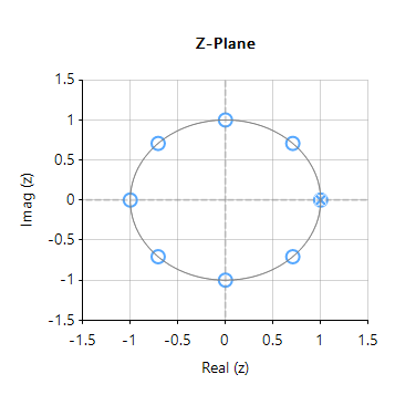
Upon initial inspection of the transfer function of Eqn. \(\small\textstyle\eqref{TF}\), it appears that the efficient Moving average filter is an IIR filter. However, analysing the pole-zero plot of the filter (shown on the right for \(\small\textstyle L=8\)), we see that the pole at DC has been cancelled by a zero, and that the resulting filter is actually an FIR filter, with the same result as Eqn. \(\small\textstyle\eqref{FIRdef}\).

Moving average filter (MA filter). It appears that the efficient MA filter is an IIR filter. However, analysing the pole-zero plot of the filter, , we see that the pole at DC has been cancelled by a zero, and that the resulting filter is actually an FIR filter, with the same result as Eqn.

Notice also that the frequency spacing of the zeros (corresponding to the nulls in the frequency response) are at spaced at \(\small\textstyle\pm\frac{Fs}{L}\). This can be readily seen for this example, where an MA of length 8, sampled at \(\small\textstyle 500Hz\), results in a \(\small\textstyle\pm62.5Hz\) resolution.

As a final point, notice that the our efficient filter requires a delay line of length \(\small\textstyle L+1\), compared with the FIR delay line of length, \(\small\textstyle L\). However, this is a small price to pay for the computation advantage of a filter just requiring one addition and one subtraction. As such, the MA filter of Eqn. \(\small\textstyle\eqref{TF}\) presented herein is very attractive for very low power processors, such as the Arm Cortex-M0 that have been traditionally overlooked for DSP operations.

Implementation

The MA filter of Eqn. \(\small\textstyle\eqref{TF}\) may be implemented in ASN FilterScript as follows:

 
ClearH1;  // clear primary filter from cascade 
interface L = {2,32,2,4}; // interface variable definition 

Main() 
Num = {1,zeros(L-1),-1}; // define numerator coefficients 
Den = {1,-1}; // define denominator coefficients 
Gain = 1/L; // define gain