Modern embedded processors, software frameworks and design tooling now allow engineers to apply advanced measurement concepts to smart factories as part of the I4.0 revolution.

In recent years, PM (predictive maintenance) of machines has received great attention, as factories look to maximise their production efficiency while at the same time retaining the invaluable skills of experienced foremen and production workers.
Traditionally, a foreman would walk around the shop floor and listen to the sounds a machine would make to get an idea of impending failure. With the advent of I4.0 AIoT technology, microphones, edge DSP algorithms and ML may now be employed in order to ‘listen’ to the sounds a machine makes and then make a classification and prediction.
One of the major challenges is how to make a computer hear like a human. In this article we will discuss how sound weighting curves can make a computer hear like a human, and how they can be deployed to an Arm Cortex-M microcontroller for use in an AIoT application.
Physics of the human ear
An illustration of the human ear shown below. As seen, the basic task of the ear is to translate sound (air vibration) into electrical nerve impulses for the brain to interpret.
The ear achieves this via three bones (Stapes, Incus and Malleus) that act as a mechanical amplifier for vibrations received at the eardrum. These amplified sounds are then passed onto the Cochlea via the Oval window (not shown).
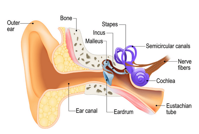
The Cochlea (shown in purple) is filled with a fluid that moves in response to the vibrations from the oval window. As the fluid moves, thousands of nerve endings are set into motion. These nerve endings transform sound vibrations into electrical impulses that travel along the auditory nerve fibres to the brain for analysis.
Modelling perceived sound
Due to complexity of the fluidic mechanical construction of the human auditory system, low and high frequencies are typically not discernible. Researchers over the years have found that humans are most perceptive to sounds in the 1-6kHz range, although this range varies according to the subject’s physical health.
This research led to the definition of a set of weighting curves: the so-called A, B, C and D weighting curves, which equalises a microphone’s frequency response. These weighting curves aim to bring the digital and physical worlds closer together by allowing a computerised microphone-based system to hear like a human.
The A-weighing curve is the most widely used as it is mandated by IEC-61672 to be fitted to all sound level meters. The B and D curves are hardly ever used, but C-weighting may be used for testing the impact of noise in telecoms systems.
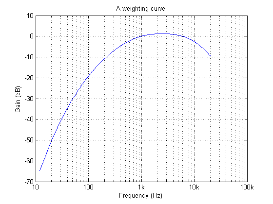
The frequency response of the A-weighting curve is shown above, where it can be seen that sounds entering our ears are de-emphasised below 500Hz and are most perceptible between 0.5-6kHz. Notice that the curve is unspecified above 20kHz, as this exceeds the human hearing range.
ASN FilterScript
ASN’s FilterScript symbolic math scripting language offers designers the ability to take an analog filter transfer function and transform it to its digital equivalent with just a few lines of code.
The analog transfer functions of the A and C-weighting curves are given below:
\(H_A(s) \approx \displaystyle{7.39705×10^9 \cdot s^4 \over (s + 129.4)^2\quad(s + 676.7)\quad (s + 4636)\quad (s + 76655)^2}\)
\(H_C(s) \approx \displaystyle{5.91797×10^9 \cdot s^2\over(s + 129.4)^2\quad (s + 76655)^2}\)
These analog transfer functions may be transformed into their digital equivalents via the bilinear() function. However, notice that \(H_A(s) \) requires a significant amount of algebracic manipulation in order to extract the denominator cofficients in powers of \(s\).
Convolution
A simple trick to perform polynomial multiplication is to use linear convolution, which is the same algebraic operation as multiplying two polynomials together. This may be easily performed via FilterScript’s conv() function, as follows:
y=conv(a,b);
As a simple example, the multiplication of \((s^2+2s+10)\) with \((s+5)\), would be defined as the following three lines of FilterScript code:
a={1,2,10};
b={1,5};
y=conv(a,b);
which yields, 1 7 20 50 or \((s^3+7s^2+20s+50)\)
For the A-weighting curve Laplace transfer function, the complete FilterScript code is given below:
ClearH1;  // clear primary filter from cascade

Main() // main loop

a={1, 129.4};
b={1, 676.7};
c={1, 4636};
d={1, 76655};

aa=conv(a,a); // polynomial multiplication
dd=conv(d,d);

aab=conv(aa,b);
aabc=conv(aab,c);

Na=conv(aabc,dd);
Nb = {0 ,0 , 1 ,0 ,0 , 0, 0}; // define numerator coefficients
G = 7.397e+09; // define gain

Ha = analogtf(Nb, Na, G, "symbolic");
Hd = bilinear(Ha,0, "symbolic");

Num = getnum(Hd);
Den = getden(Hd);
Gain = getgain(Hd)/computegain(Hd,1e3);    // set gain to 0dB@1kHz
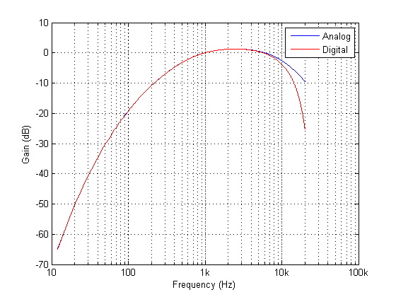
Frequency response of analog vs digital A-weighting filter for \(f_s=48kHz\). As seen, the digital equivalent magnitude response matches the ideal analog magnitude response very closely until \(6kHz\).
The ITU-R 486–4 weighting curve
Another weighting curve of interest is the ITU-R 486–4 weighting curve, developed by the BBC. Unlike the A-weighting filter, the ITU-R 468–4 curve describes subjective loudness for broadband stimuli. The main disadvantage of the A-weighting curve is that it underestimates the loudness judgement of real-world stimuli particularly in the frequency band from about 1–9 kHz.
Due to the precise definition of the 486–4 weighting curve, there is no analog transfer function available. Instead the standard provides a table of amplitudes and frequencies – see here. This specification may be directly entered into FilterScript’s firarb() function for designing a suitable FIR filter, as shown below:
ClearH1;  // clear primary filter from cascade
ShowH2DM;

interface L = {10,400,10,250}; // filter order

Main()

// ITU-R 468 Weighting
A={-29.9,-23.9,-19.8,-13.8,-7.8,-1.9,0,5.6,9,10.5,11.7,12.2,12,11.4,10.1,8.1,0,-5.3,-11.7,-22.2};
F={63,100,200,400,800,1e3,2e3,3.15e3,4e3,5e3,6.3e3,7.1e3,8e3,9e3,1e4,1.25e4,1.4e4,1.6e4,2e4};

A={-30,A};  //  specify arb response
F={0,F,fs/2};

Hd=firarb(L,A,F,"blackman","numeric");

Num=getnum(Hd);
Den={1};
Gain=getgain(Hd);
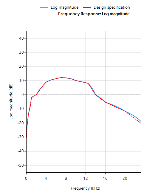
firarb() function for \(f_s=48kHz\)As seen, FilterScript provides the designer with a very powerful symbolic scripting language for designing weighting curve filters. The following discussion now focuses on deployment of the A-weighting filter to an Arm based processor via the tool’s automatic code generator. The concepts and steps demonstrated below are equally valid for FIR filters.
Automatic code generation to Arm processor cores via CMSIS-DSP
The ASN Filter Designer’s automatic code generation engine facilitates the export of a designed filter to Cortex-M Arm based processors via the CMSIS-DSP software framework.
The tool’s built-in analytics and help functions assist the designer in successfully configuring the design for deployment. Professional licence users may expedite the deployment by using the Arm deployment wizard that automates the steps described below.
Steps required for Educational licence users only
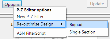
Before generating the code, the H2 filter (i.e. the filter designed in FilterScript) needs to be firstly re-optimised (transformed) to an H1 filter (main filter) structure for deployment. The options menu can be found under the P-Z tab in the main UI.
All floating point IIR filters designs must be based on Single Precision arithmetic and either a Direct Form I or Direct Form II Transposed filter structure. The Direct Form II Transposed structure is advocated for floating point implementation by virtue of its higher numerically accuracy.
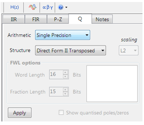
Quantisation and filter structure settings can be found under the Q tab (as shown on the left). Setting Arithmetic to Single Precision and Structure to Direct Form II Transposed and clicking on the Apply button configures the IIR considered herein for the CMSIS-DSP software framework.
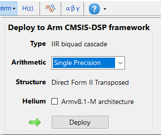
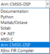
Select the Arm CMSIS-DSP framework from the selection box in the filter summary window:
The automatically generated C code based on the CMSIS-DSP framework for direct implementation on an Arm based Cortex-M processor is shown below:
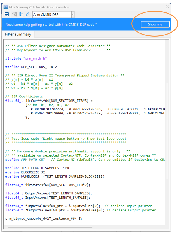
As seen, the ASN Filter Designer’s automatic code generator generates all initialisation code, scaling and data structures needed to implement the A-weighting filter IIR filter via Arm’s CMSIS-DSP library. A detailed help tutorial is available by clicking on the Show me button.