Many IoT applications use a sinewave for estimating the amplitude of an entity of interest – some examples include:
- Measuring material fatigue/strain with a loadcell – in vehicle and bridge/building applications measuring material fatigue and strain is essential for safety. An AC sinusoidal excitation overcomes the difficulty of dealing with instrumentation electronics DC offsets.
- Calibrating CT (current transformers) sensors channels – a sinusoid of known amplitude is applied to channel input and the output amplitude is measured.
- Measuring gas concentration in infra-red gas sensors – the resulting sinusoid’s amplitude is used to provide an estimate of gas concentration.
- Measuring harmonic amplitudes in power quality smart grids applications – in 50/60Hz power systems, certain harmonic amplitudes are of interest.
- ECG biomedical compliance testing – channel compliance with IEC regulations needed for FDA testing typically uses a set of sinewaves at known amplitudes, to ensure that the channel amplitude error is within specification.
In a previous article, we discussed how differentiation could be used to find the peaks and troughs of sinewave, i.e. finding the zero crossing points. However, a much more traditional approach has been to use fullwave rectification, whereby a non-linear operator and lowpass filtering are employed. The concept used is described below:
- Remove any DC or low-frequency offsets via a highpass filter.
- Apply a non-linear operator via an abs() or sqr() non-linear operator.
- Lowpass filter the result to obtain an estimate of the sinusoid’s amplitude.
- Scale the amplitude.
Although this sounds easy, care should be taken to understand the effects of how the non-linear operator alters the waveform and affects the estimation of amplitude using lowpass filtering.
IoT application
A typical IoT application using a sinusoid is shown below:
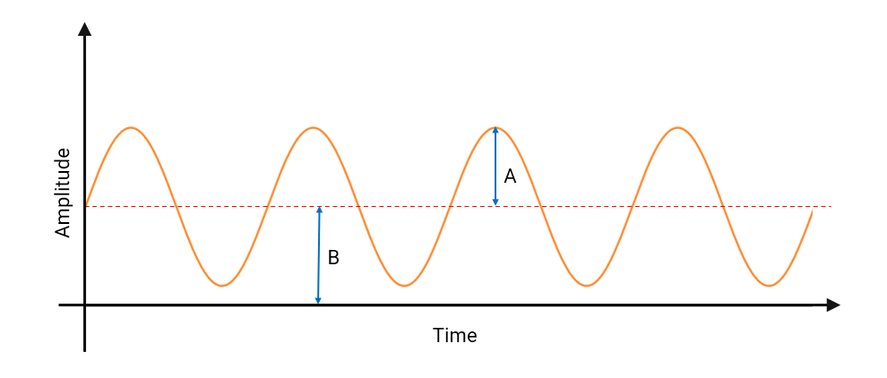
As seen, the waveform can be modelled as:
\(x\left(n\right)=A\,sin\left(2\pi f_ot\right)+B\)
Where, \(f_o\) is the frequency of oscillation and \(A\) is the amplitude of sinusoid respectively. Notice that the sinusoid is non-linear and symmetrical around the offset, \(B\). Notice also that it has a peak-to-peak amplitude of \(2A\), since specifying an amplitude \(A\) results in a bipolar amplitude of \(±A\). As many microcontrollers employ low-cost unipolar ADCs, the bipolar sinusoid needs to be offset by a DC offset, \(B\) (usually achieved by a resistor network) to ensure that the signal remains within the common-mode range of the ADC input.
As mentioned above, before applying the non-linear operator any DC offsets need to be removed. This can easily be achieved with either an IIR or FIR highpass filter. If using an IIR filter, it should be noted that the filter’s phase and group delay (latency) will significantly increase at the cut-off frequency, so a degree of experimentation is required to find a good trade-off.
After highpass filtering the data, we can apply the non-linear operator. Two popular operators are the abs()and sqr() operators.
Using the abs() operator, the Fourier series of \(\left|A \,sin(2\pi f_ot)\right|\) is shown below:
\(\left|A\ sin(2\pi f_ot)\right|\ =\ \displaystyle A\left[ \frac{2}{\pi}\ -\ \displaystyle\frac{4}{\pi}\normalsize{\sum\limits_{k=1}^{\infty}}\frac{cos(4k\pi f_ot)}{4k^2-1}\right]\)
Analysing the equation, it can be seen that the abs() operation doubles the frequency and that the DC component is actually \(\frac{2A}{\pi}\), as illustrated below.
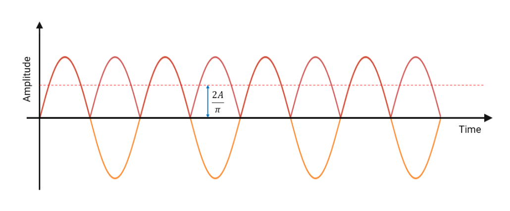
As seen, lowpass filtering this result in its current form will produce an amplitude estimate of \(\frac{2A}{\pi}\) (dashed red line), which is clearly incorrect for estimating the sinewave’s amplitude, \(A\). However, this can be simply remedied by scaling the amplitude estimates by \(\frac{\pi}{2}\), which removes the bias, leaving the sinewave’s amplitude, \(A\).
Likewise, for a sqr() operator, we can define the resulting waveform using trigonometrical identities, i.e.
\({sin^2(2\pi f_ot)}\ =\ A\left[\displaystyle\frac{1\ -\ cos(4\pi f_ot)}{2}\right]\)
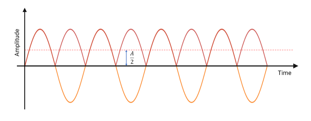
Lowpass filtering this signal requires a correction scaling factor of 2.
Lowpass filter
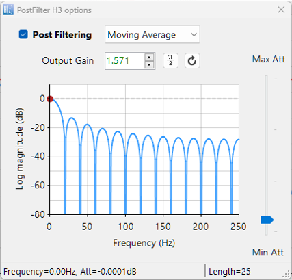
Although any lowpass filter will suffice, the moving average filter is used by most developers by virtue of its computational simplicity and noise reduction characteristics. A more detailed explanation of moving average filters can be found here.
A 24th order moving average filter with a post gain of \(\frac{\pi}{2}\) or 1.571 is shown below.
Applying this moving average filter to a sinewave \(f_o=10Hz, A=0.5\), sampled at 500Hz processed with the abs()operator we obtain the following:
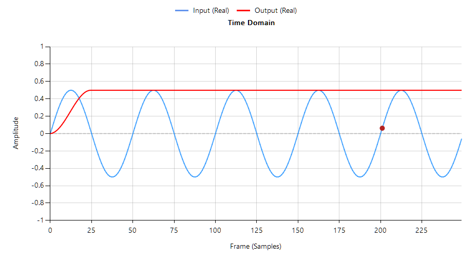
As seen, the amplitude estimation of the sinusoid using a lowpass filter and the \(\frac{\pi}{2}\) scaling factor is now correct. However, for real world applications that contain noise, it is considered to be more accurate to measure the RMS amplitude, in which case the scaling factor becomes \(\frac{\pi}{2\sqrt 2} \).
Note that these scaling factors are only valid for sinusoidal scaling. If your waveform is non-sinusoidal (e.g. triangular or square or affected by harmonics) another scaling factor/method will be required, as discussed below.
True RMS
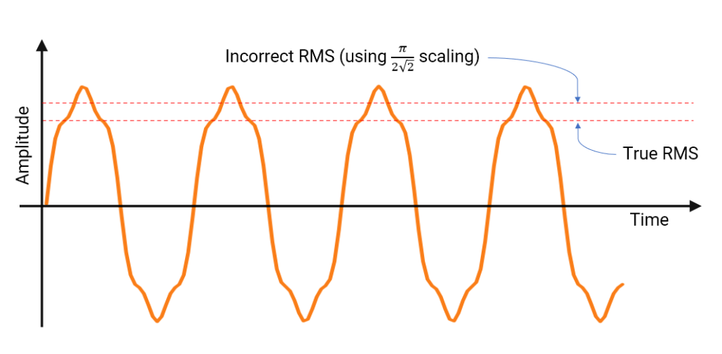
In practice, many sinusoidal waveforms will be affected by harmonics (e.g. smart grid power systems) which will alter the shape of the main sinusoid and offset the RMS estimate using the \(\frac{\pi}{2\sqrt 2} \) scaling factor concept.
A much better method is to calculate the True RMS, whereby the sqr() operator is used for the full wave rectification, but this time a sqrt() function is used for scaling after the lowpass operation. The results of the two methods are shown below, where it can be seen that the True RMS method correctly estimates the signal’s RMS amplitude.