Over the past 40 years, I’ve worked with a wide range of microcontrollers and DSPs across industries—from biomedical systems and industrial control to radar and audio processing. What follows is not theory—it’s a reflection based on firsthand experience with many of the chips and platforms that have shaped the embedded world as we know it.
Before the Age of General-Purpose DSPs
In the early 1980s, Digital Signal Processing (DSP) was often too demanding for microprocessors, which lacked the speed and specialised instruction sets. To address this, manufacturers developed dedicated hardware accelerators—custom ICs built to perform tasks such as Fast Fourier Transforms (FFT), digital filtering, and modulation. Companies such as TRW LSI Products, Harris Semiconductor and even Intel offered function-specific chips that could be dropped into hardware designs to offload processing from the main CPU. These chips laid the groundwork for programmable DSPs, which would later unify these capabilities into a single, software-controlled processor—offering far greater flexibility and reusability.
The Three Titans of Classic DSP: TI, Analog Devices and Motorola
Back in the golden age of classic DSPs, three companies stood out: Texas Instruments, Analog Devices, and Motorola. Each brought its own innovations, architectures, and ecosystems that defined digital signal processing for decades.
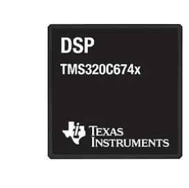
Texas Instruments (TI) took the lead with its TMS320 family. Initially introduced in 1983, the fixed-point TMS32010 was one of the first general-purpose DSPs on the market. TI’s later C2000 series brought DSP-like performance to microcontrollers—making it a popular choice for motor control and industrial automation. But it was the TMS320C6000 series, launched in the late 1990s, that truly set a new benchmark. These VLIW (Very Long Instruction Word) DSPs—such as the C62x (fixed-point) and C67x (floating-point)—enabled complex signal analysis, control, and real-time processing with high instruction throughput.Later multicore versions like the C6474 scaled this up with three high-performance DSP cores on a single chip. Some designs even scaled to six cores in custom implementations. These chips made it possible to perform real-time control, sensor fusion, and high-throughput signal analysis in a way that felt almost futuristic —achieving over 28,000 MIPS!
TI also addressed ultra-low-power use cases with the C55x series—a fixed-point DSP line optimised for battery-powered audio and telecommunication applications. Whether for performance or power efficiency, TI had an answer across the spectrum.
Analog Devices (ADI) also played a central role in shaping DSP. Their SHARC and TigerSHARC families offered high-performance floating-point computation, making them a favourite in professional audio, instrumentation, and aerospace applications. Equally important was the Blackfin family—a fixed-point, 16/32-bit hybrid architecture introduced in the early 2000s. Blackfin was optimised for embedded multimedia and signal processing tasks, combining DSP capability with control-oriented features like MMUs, timers, and flexible I/O. ADI offered excellent tools, tight integration with analog components, and very strong real-time performance for demanding applications.
Motorola, meanwhile, contributed both microcontroller and DSP innovations. The legendary 68000, launched in 1979, wasn’t strictly a DSP, but it offered 32-bit general-purpose performance that was far ahead of its time. It was widely adopted in embedded control systems and even some signal processing applications—powering everything from defence platforms to the Commodore Amiga. Motorola also developed a dedicated line of DSPs in the 56000 family, which gained a following in telecommunications and audio. Eventually, Motorola spun off its semiconductor business as Freescale, and later moved to PowerPC architectures. Still, its legacy in early DSP computing remains significant.
Collectively, these three vendors established the blueprint for programmable signal processing—offering both fixed-point and floating-point variants, with increasing performance, integration, and software support over time. Their contributions laid the groundwork for today’s hybrid processors, SoCs, and enhanced microcontrollers.
Enter Microchip’s dsPIC: A Different Kind of DSP
When Microchip launched the dsPIC series in 2001, it was a radical departure from the classic DSP playbook. Instead of focusing on high-performance signal processing, Microchip blended DSP-like instructions into a 16-bit microcontroller core—creating a hybrid that prioritised real-time control, affordability, and embedded peripherals all-in-one. This unorthodox approach defied convention, yet proved surprisingly effective in areas such as motor control and power electronics.
In 2007, Microchip introduced the PIC32, a 32-bit fixed-point MIPS architecture intended to compete with Arm-based microcontrollers. Floating-point support only arrived in PIC32MZ devices in 2013, which still retained the MIPS lineage. By then, the industry had largely moved on. After acquiring Atmel in 2016, Microchip began transitioning toward Arm-based designs—but found themselves playing catch-up. STMicroelectronics, NXP, and others had already embraced Arm more than a decade earlier.
Hitachi and the SH Architecture
Another important player in the 1990s was Hitachi, whose SuperH (SH) family of microcontrollers gained traction in both consumer electronics and automotive systems. The SH architecture offered a compact 32-bit RISC instruction set and DSP-like instructions, making it well-suited for signal processing tasks without the complexity of a full DSP.
The SH-2, in particular, was developed for motor control and stood out for its high performance and nicely designed 32-bit architecture. It was backed by a professional-grade toolchain—more expensive than Microchip’s offerings, and far more capable. While Microchip’s later dsPIC family also targeted fixed-point DSP applications, it was positioned more toward the hobbyist and cost-sensitive market. In contrast, the SH-2 catered to industrial and automotive use cases that demanded greater precision, performance, and software maturity.
The SH line powered everything from set-top boxes and printers to game consoles, with the SH-2 used in the Sega Saturn and the more powerful SH-4 driving the Sega Dreamcast. After merging with Mitsubishi’s semiconductor division to form Renesas in 2003, the SH series continued for a while but was gradually replaced by newer architectures such as RX and eventually Arm-based cores. Nonetheless, the SH family remains a fascinating example of early DSP-capable microcontrollers.
How Arm Processors Changed the Game
The real turning point for Arm came in 1995, when they secured a major contract with Nokia. At the time, Nokia was searching for a low-power processor for its mobile phones—something that could offer signal processing without the power drain of conventional DSPs.
Arm responded with the Thumb instruction set—a compact 16-bit format that dramatically reduced code size while preserving much of the performance of 32-bit Arm instructions. Later, Thumb-2 extended this approach with mixed 16/32-bit support, enabling DSP-like functionality within a power-efficient and compact silicon footprint. It was a game-changer.
However, what truly propelled Arm forward was its strategy and licensing model. Rather than manufacturing chips themselves, Arm licensed its processor IP to silicon vendors—forming deep partnerships with companies such as STMicroelectronics, NXP, Texas Instruments, and Analog Devices. These vendors integrated Arm cores into their own SoCs, often alongside analog front ends, accelerators, or even DSP blocks. The result was a wave of highly optimised, application-specific devices built atop a shared architecture.
A key milestone came with Broadcom’s adoption of the Cortex-A family, which powered the first Raspberry Pi. The Pi’s success brought Arm processors into education, prototyping, and hobbyist markets—seeding a new generation of developers trained on Arm platforms.
Combined with a robust ecosystem of compilers, development tools, and middleware, Arm’s architectural dominance spread rapidly across consumer, industrial, and IoT domains.
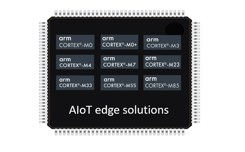
The Emergence of the Enhanced Microcontroller
Today’s microcontrollers are far more than just control engines. Many now include SIMD instructions, DSP acceleration, advanced timers, cryptographic modules, and hardware-based security. This gives rise to what might be called the enhanced microcontroller—a class of devices that blur the line between DSPs and MCUs.
Today’s microcontrollers are no longer just simple control devices. Many now include SIMD instructions, DSP acceleration, and hardware-based security. This gives rise to what we can call the enhanced microcontroller—a hybrid class that combines:
- General-purpose control and peripheral integration
- DSP capabilities for signal conditioning and real-time analysis
- Hardware security features such as TrustZone
- Low power consumption for battery-powered and IoT systems
- Affordable pricing for mass deployment
STMicroelectronics’ STM32 family—based on Cortex-M4 and M7 cores—is a textbook example. These microcontrollers can handle filtering, FFTs, and real-time signal analysis with ease, all while supporting familiar C-based toolchains and low-power sleep modes. They may not match a high-end floating-point DSP in every respect, but they strike an ideal balance for most embedded applications.
Arm Helium: Specialised Edge Hardware Acceleration
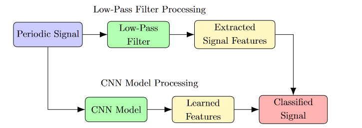
Arm Helium—also known as the Armv8.1-M Scalable Vector Extension (MVE)—takes this trend a step further. Designed for edge AI, Helium allows microcontrollers to perform complex filtering, sensor fusion, and even neural inference tasks with impressive efficiency.
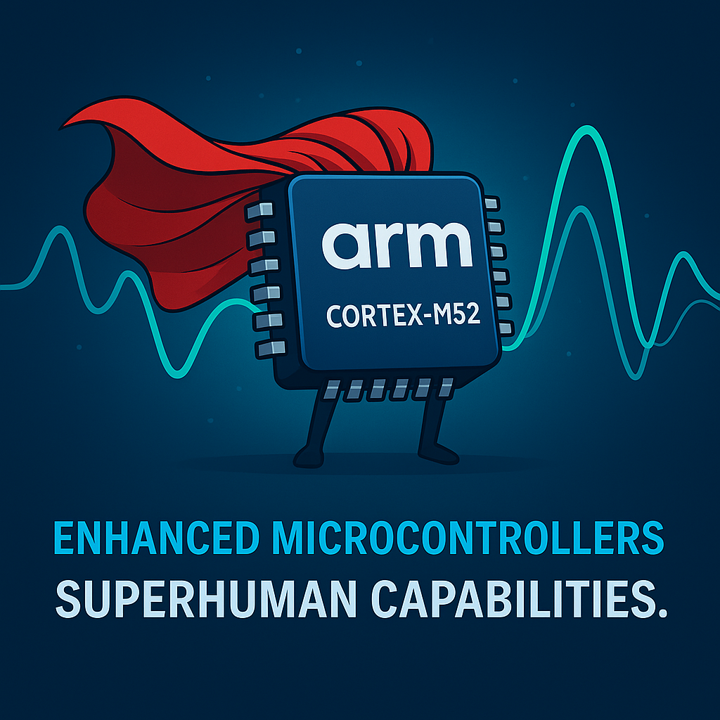
The Cortex-M52 captures the essence of this shift—bringing DSP, general-purpose control, security, and low-power performance together into a single core. It introduces Arm TrustZone for embedded security, supports Helium acceleration, and enables localised processing of tasks that once required external compute or specialised DSPs.
Many new Helium-based MCUs also leverage TSMC’s 22nm ultra-low-power process, delivering up to 50% power savings over 40nm chips. This makes edge intelligence viable even in battery- or solar-powered deployments, with no compromise on performance.
It’s Not Just the Hardware—It’s the Ecosystem
Arm’s success is also rooted in the richness of its ecosystem. Developers benefit from mature toolchains, CMSIS-DSP libraries, trusted third-party support, and a wide community of contributors.
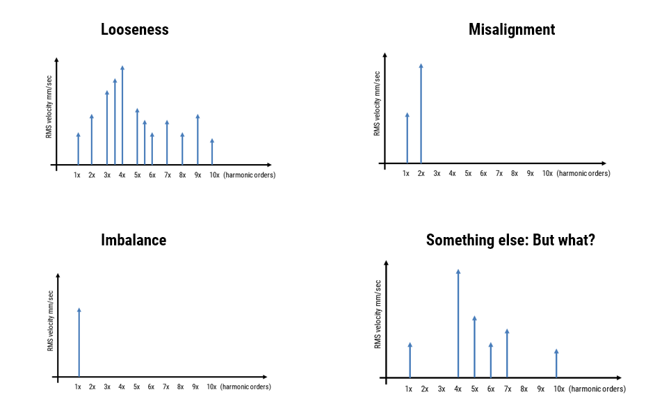
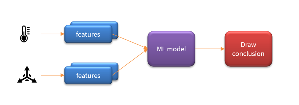
This infrastructure allows engineers to focus on solving domain-specific problems rather than wrestling with the underlying hardware. Thanks to tools from ASN, Qeexo, Mathworks and Edge Impulse even sophisticated algorithms—such as biomedical filters, IoT sensor cleaning filters, and predictive maintenance monitors—can now be designed, validated, and deployed as efficient C code within minutes, without requiring deep DSP expertise.
Arm’s ecosystem lowers the entry barrier while raising the ceiling, enabling individual developers and small teams to compete with traditional DSP engineering departments. It’s this accessibility and scalability that makes the platform so compelling for modern embedded development.
Enter the Market Disruptor: Espressif Semiconductor
While much of the evolution in embedded DSP has been driven by microcontrollers based on Arm-Cortex cores from vendors such as STMicroelectronics, Texas Instruments, Analog Devices and NXP, a disruptive force entered the scene in 2016 with the launch of Espressif Semiconductor’s ESP32-WROOM-32.
Based on dual-core Xtensa® 32-bit LX6 processors, the original ESP32 combines integrated Wi-Fi and Bluetooth with a hardware single-precision floating-point unit (FPU) and DSP-style instructions such as multiply-accumulate and saturation arithmetic. Despite lacking hardware support for division and square root, its real-world floating-point performance is often comparable to an Arm Cortex-M4F, thanks to its 240 MHz clock and efficient memory architecture.
Originally aimed at wireless control applications, the ESP32 quickly gained traction for low-cost edge processing tasks—including audio filtering, FFT analysis, and real-time control. Espressif’s open SDK and active global community positioned it as the go-to resource for hobbyists, start-ups, and even commercial IoT products.
While it lacks the advanced DSP acceleration of Arm Helium or the precision of high-end floating-point DSPs, the ESP32’s exceptional cost-to-performance ratio has democratised edge intelligence. It has showed the world that embedded DSP doesn’t have to be expensive or exclusive.
Where Do We Stand Now?
DSP has not disappeared—it has evolved. What was once the domain of dedicated chips has become a fundamental capability, embedded across a wide range of computing platforms. From soft DSP cores in FPGAs to integrated signal processing units in SoCs, and now to scalable vector extensions within microcontrollers, the function of DSP is alive and well—although the form has changed.
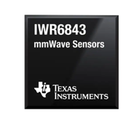
Specialist chips, such as those from Texas Instruments or Analog Devices, have not vanished. Many are now integrated into SoCs—handling radar, video, and high-performance industrial tasks in highly integrated systems. The IWR6834 mmwave radar SoC from TI is a perfect example of this convergence: a C674x floating point DSP, two Arm Cortex-R4 processors, communication channels, memory, RF frontend, and antennas all in one compact, high-performance chip. Newer flavours of the SoC, include an AI engine for micro-doppler pattern classification. All of which can be inferenced at the edge in real-time!
However, for most embedded applications, enhanced microcontrollers based on Arm processors now deliver the best balance of performance, power, and price. With integrated support for signal processing, connectivity, security, and energy efficiency—all within a mature ecosystem—they have become the logical choice for the next generation of intelligent edge devices.
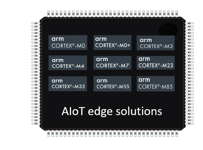
Across the Cortex-M family, options like the M4 and M7 provide a strong foundation for signal processing in real-time control applications. The Helium-enabled M55, M85, and most recently the M52, take this further—offering vectorised DSP acceleration, better energy efficiency, and increasingly robust security features.
The Cortex-M52 in particular captures the essence of this evolution. It unifies three essential capabilities for Edge AI into one compact, low-power device:
- DSP/AI functionality for signal processing algorithms, such as filtering and feature extraction, and running ML models
- Low power consumption to enable battery or energy-harvesting applications
- Hardware-based security, including Arm TrustZone, to safeguard code and data
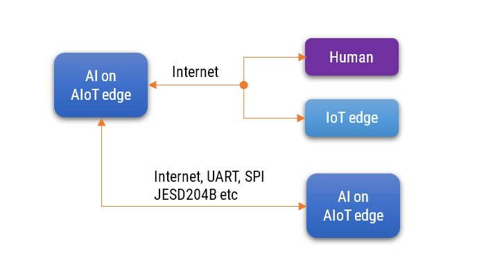
This convergence enables true Real-Time Edge Intelligence (RTEI)—where signals are captured, interpreted, and acted upon locally, without relying on cloud infrastructure or external accelerators. Tasks such as biomedical filtering, sensor fusion, anomaly detection, and embedded inference can now be performed directly at the edge, at a fraction of the power and cost of what was previous required.
And with newer devices manufactured on advanced low-power nodes—such as TSMC’s 22nm process—power consumption is reduced by up to 50% compared to older 40nm designs. This makes the deployment of smart, responsive, and secure edge systems more sustainable and scalable than ever before.
And today, over 90% of all microcontrollers use an Arm core, which is a testament to Arm’s rich ecosystem and proven technologies.
This is not just a shift in hardware—it’s a redefinition of where and how computing happens in the embedded world of 2025 and beyond. It happens in real time, at the edge.