Upgrading legacy designs based on analog filters
Analog filters have been around since the beginning of electronics, ranging from simple inductor-capacitor networks to more advanced active filters with op-amps. As such, there is a rich collection of tried and tested legacy filter designs for a broad range of sensor measurement applications. However, with the performance requirements of modern IoT (Internet of Things) sensor measurement applications and lower product costs, digital filters integrated into the microcontroller’s application code are becoming the norm, but how can we get the best of both worlds?
Rather than re-inventing the wheel, product designers can take an existing analog filter transfer function, transform it to digital (via a transform) and implement it as digital filter in a microcontroller or DSP (digital signal processor). Although analog-to-digital transforms have been around for decades, the availability of DSP design tooling for tweaking the ‘transformed digital filter’ has been somewhat limited, hindering the design and validation process.
A 2nd order analog lowpass filter is shown below, and in its simplest form, only 5 components are required to build the filter, which sounds easy. Right?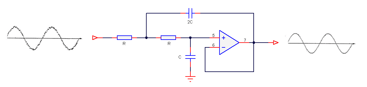
The pros
The most obvious advantage is that analog filters have an excellent resolution, as there are no ‘number of bits’ to consider. Analog filters have good EMC (electromagnetic compatibility) properties as there is no clock generating noise. There are no effects of aliasing, which is certainly true for the simpler op-amps, which don’t have any fancy chopping or auto-calibration circuitry built into them, and analog designs can be cheap which is great for cost sensitive applications.
Sound great, but what’s the bad news?
Analog filters have several significant disadvantages that affect filter performance, such as component aging, temperature drift and component tolerance. Also, good performance requires good analog design skills and good PCB (printed circuit board) layout, which is hard to find in the contemporary skills market.
These disadvantages make digital filters much more attractive for modern applications, that require high repeatability of characteristics. Looking at an example, let’s say that you want to manufacture 1000 measurement modules after optimising your filter design. With a digital solution you can be sure that the performance of your filter will be identical in all modules. This is certainly not the case with analog, as component tolerance, component aging and temperature drift mean that each module’s filter will have its own characteristics. Also, an analog filter’s frequency response remains fixed, i.e. a Butterworth filter will always be a Butterworth filter – any changes the frequency response would require physically changing components on the PCB – not ideal!
Digital filters are adaptive and flexible, we can design and implement a filter with any frequency response that we want, deploy it and then update the filter coefficients without changing anything on the PCB! It’s also easy to design digital filters with linear phase and at very low sampling frequencies – two things that are tricky with analog.
Laplace to discrete/digital transforms
The three methods discussed herein essentially involve transforming a Laplace (analog) transfer function, \(H(s)\) into a discrete transfer function, \(H(z)\) such that a tried and tested analog filter that is already used in a design may be implemented on a microcontroller or DSP.
A selection of some useful Laplace to z-transforms are given in table below:
\(
\begin{array}{ccc}\hline
H(s) &\longleftrightarrow & H(z) \\ \hline
1 &\longleftrightarrow & 1 \\
\frac{\displaystyle1}{\displaystyle s}
&\longleftrightarrow& \frac{\displaystyle 1}{\displaystyle 1-z^{\scriptstyle -1}}\\
\frac{\displaystyle 1}{\displaystyle s^{\scriptstyle 2}} &\longleftrightarrow& \frac{\displaystyle
Tz^{\scriptstyle-1}}{\displaystyle (1-z^{\scriptstyle -1})^2}\\
\frac{\displaystyle 1}{\displaystyle s+a}
&\longleftrightarrow&
\frac{\displaystyle 1}{\displaystyle 1-e^{-aT}z^{-1}}\\
\frac{\displaystyle 1}{\displaystyle (s+a)^2}
&\longleftrightarrow& \frac{\displaystyle z^{-1}(1-e^{-aT})}{\displaystyle a(1-z^{-1})(1-e^{-aT}z^{-1})}\\\hline
\end{array}
\)
A table of useful Laplace and z-transforms
The Bilinear z-transform (BZT)
The Bilinear z-transform (BZT), simply converts an analog transfer function, \(H(s)\) into a discrete transfer function, \(H(z)\) by replacing all \(s\) terms with the following:
\(\displaystyle
s=\frac{2}{T}\frac{1-z^{-1}}{1+z^{-1}} \label{bzt}\)
where, \(T\) is the discrete system’s sampling period. However, substituting \(s=j\Omega\) and \(z=e^{jwT}\) into the BZT equation and simplifying, notice that there is actually a non-linear relationship between the analog, \(\Omega\) and discrete, \(w\) frequencies. This relationship is shown below, and is due to the nonlinearity of the arctangent function.
\(\displaystyle\omega=2\tan^{-1}\left(\frac{\Omega T}{2}\right)\label{bzt_warp_def1}\)
Analysing the equation, it can be seen that the equally spaced analog frequencies in the range \( -\infty\lt\Omega\lt\infty\) are nonlinearly compressed in the frequency range \( -\pi\lt w\lt\pi\) in the discrete domain. This relationship is referred to as frequency warping, and may be compensated for by pre-warping the analog frequencies by:
\(\displaystyle
\Omega_c=\frac{2}{T}\tan\left(\frac{\Omega_d T}{2}\right)
\label{bzt_warp_def2}
\)
where, \(\displaystyle\Omega_c\) is the compensated or pre-warped analog frequency, and \(\displaystyle\Omega_d\) is the desired analog frequency.
The ASN FilterScript command \(\texttt{bilinear}\) may be used convert a Laplace transfer function into its discrete equivalent using the BZT transform. An example is given below.
The Impulse Invariant Transform
The second transform, is referred to as the impulse invariant transform (IIT), since the poles of the Laplace transfer function are converted into their discrete equivalents, such that the discrete impulse response, \(h(n)\) is identical to a regularly sampled representation of the analog impulse response (i.e., \(h(n)=h(nT)\), where \(T\) is the sampling rate, and \(t=nT\)). The IIT is a much more tedious transformation technique than the BZT, since the Laplace transfer function must be firstly expanded using partial fractions before applying the transform.
The transformation technique is defined below:
\(\displaystyle
\frac{K}{s+a} \quad\longrightarrow\quad
\frac{K}{1-e^{-aT}z^{-1}} \label{iit_def}
\)
This method suffers from several constraints, since it does not allow for the transformation of zeros or individual constant terms (once expanded), and must have a high sampling rate in order to overcome the effects of spectral aliasing. Indeed, the effects of aliasing hinder this method considerably, such that the method should only be used when the requirement is to match the analog transfer function’s impulse response, since the resulting discrete model may have a different magnitude and phase spectrum (frequency response) to that of the original analog system. Consequently, the impulse invariant method is unsuitable for modelling highpass filters, and is therefore limited to the modelling of lowpass or bandpass type filters.
Due to the aforementioned limitations of the IIT method, it is currently not supported in ASN Filterscript.
The Matched-z transformation
Another analog to discrete modelling technique is the matched-z transformation. As the name suggests, the transform converts the poles and zeros from the analog transfer function directly into poles and zeros in the z-plane. The transformation is described below, where \(T\) is the sampling rate.
\(\displaystyle
\frac{\prod\limits_{k=1}^q(s+b_k)}{\prod\limits_{k=1}^p(s+a_k)}
\quad\longrightarrow\quad
\frac{\prod\limits_{k=1}^q(1-e^{-b_kT}z^{-1})}{\prod\limits_{k=1}^p(1-e^{-a_kT}z^{-1})}
\label{matchedz_def}
\)
Analysing the transform equation, it can be seen that the transformed z-plane poles will be identical to the poles obtained with the impulse invariant method. However, notice that the positions of the zeros will be different, since the impulse invariant method cannot transform them.
The ASN Filterscript command \(\texttt{mztrans}\) is available for this method.
A detailed example
In order to demonstrate the ease of transforming analog filters into their discrete/digital equivalents using the analog to discrete transforms, an example of modelling with the BZT will now follow for a 2nd order lowpass analog filter.
A generalised 2nd order lowpass analog filter is given by:
\(\displaystyle
H(s)=\frac{w_c^2}{s^2+2\zeta w_c s + w_c^2}
\)
where, \(w_c=2\pi f_c\) is the cut-off frequency and \(\zeta\) sets the damping of the filter, where a \(\zeta=1/\sqrt{2}\) is said to be critically damped or equal to -3dB at \(w_c\). Many analog engineers choose to specify a quality factor, \(Q = \displaystyle\frac{1}{2\zeta}\) or peaking factor for their designs. Substituting \(Q\) into \(H(s)\), we obtain:
\(\displaystyle
H(s)=\frac{w_c^2}{s^2+ \displaystyle{\frac{w_c}{Q}s} + w_c^2}
\)
Analysing, \(H(s)\) notice that \(Q=1/\sqrt{2} = 0.707\) also results in a critically damped response. Various values of \(Q\) are shown below, and as seen when \(Q>1/\sqrt{2}\) peaking occurs.
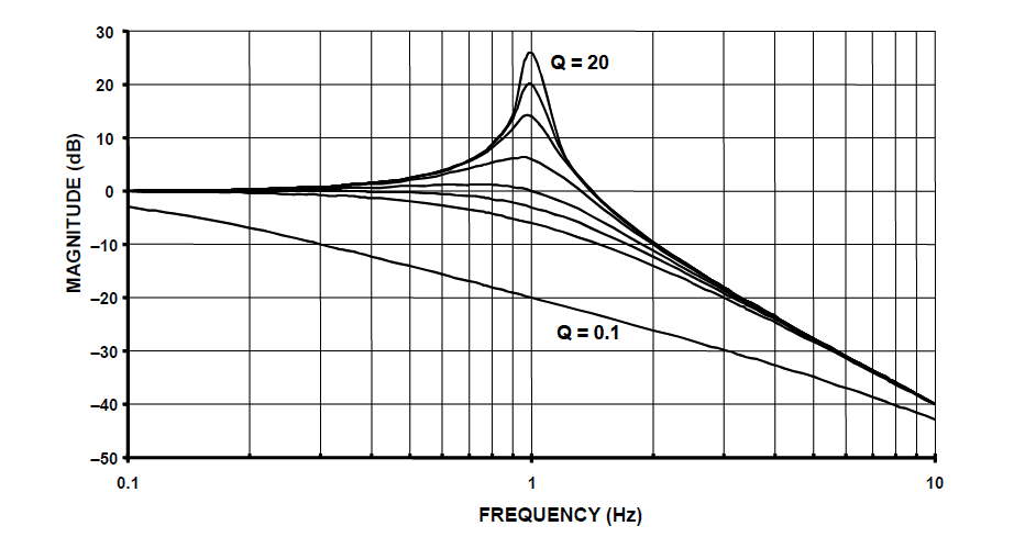
2nd order lowpass filter prototype magnitude spectrum for various value of Q:
notice that when \(Q>1/\sqrt{2}\) peaking occurs.
Before applying the BZT in ASN FilterScript, the analog transfer function must be specified in an analog filter object. The following code sets up an analog filter object for the 2nd order lowpass prototype considered herein:
[code language=”java”]
Main()
wc=2*pi*fc;
Nb={0,0,wc^2};
Na={1,wc/Q,wc^2};
Ha=analogtf(Nb,Na,1,"symbolic"); // make analog filter object
[/code]
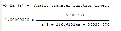
The \(\texttt{symbolic}\) keyword generates a symbolic transfer function representation in the command window. For a sampling rate of \(f_s=500Hz\) and \(f_c=30Hz\) and \(Q=0.707\), we obtain:
Applying the BZT via the \(\texttt{bilinear}\) command without prewarping,
[code language=”java” light=”true”] Hd=bilinear(Ha,0,"symbolic"); [/code]
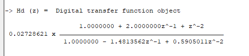
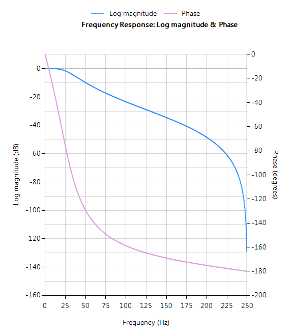
The complete frequency response of the transformed digital filter is shown below, where it can be seen that the at \(30Hz\) the magnitude is \(-3dB\) and the phase is \( -90^{\circ}\), which is as expected. Notice also how the filter’s magnitude roll-off is affected by the double zero pair at Nyquist (see the z-plane chart below), leading to differences from its analog cousin. 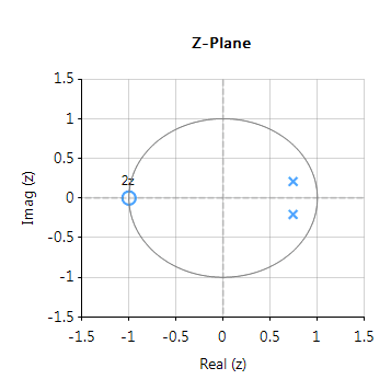
The pole-zero positions may be tweaked within ASN Filterscript or via the ASN Filter Designer’s interactive pole-zero z-plane plot editor by just using the mouse!
Implementation
The complete code for transforming a generalised 2nd order analog lowpass filter prototype into its digital equivalent using the BZT via ASN FilterScript is given below:
[code language=”java”]
ClearH1; // clear primary filter from cascade
interface Q = {0.1,10,0.02,0.707};
interface fc = {10,200,10,40};
Main()
wc=2*pi*fc;
Nb={0,0,wc^2};
Na={1,wc/Q,wc^2};
Ha=analogtf(Nb,Na,1,"symbolic"); // make analog filter object
Hd=bilinear(Ha,0,"symbolic"); // transform Ha via BZT into digital object, Hd
Num=getnum(Hd);
Den=getden(Hd);
Gain=getgain(Hd);
[/code]