In recent years, major microcontroller IC vendors such as: ST, NXP, TI, ADI, Atmel/Microchip, Cypress, Maxim to name but a few have based their modern 32-bit microcontrollers on Arm’s Cortex-M processor cores. This exciting trend means that algorithms traditionally undertaken in expensive DSPs (digital signal processors) can now be integrated into a powerful low-cost and power efficient microcontroller packed full of a rich assortment of connectivity and peripheral options, which is ideal for many IoT applications.
For many IC vendors, the coupling of DSP functionality with the flexibility of a low power microcontroller, has allowed them to offer their customers a generation of so called 32-bit enhanced microcontrollers suitable for a variety of practical applications. More importantly, this marriage of technologies has also allowed designers working on price critical IoT applications to implement complex algorithmic concepts, while at the same time keeping the overall product cost low and still achieving excellent low power performance.
Upgrading legacy analog filters with the ASN Filter Designer
Analog filters have been around since the beginning of electronics, ranging from simple inductor-capacitor networks to more advanced active filters with op-amps. As such, there is a rich collection of tried and tested legacy filter designs for a broad range of sensor measurement applications.
ASN’s FilterScript symbolic math scripting language offers designers the ability to take an existing analog filter transfer function and transform it to digital with just a few lines of code. The ASN Filter Designer’s Arm automatic code generator analyses the designed digital filter and then automatically generates Arm CMSIS-DSP compliant C code suitable for direct implementation on a Cortex-M based microcontroller.
Arm CMSIS-DSP software framework
The Arm CMSIS-DSP (Cortex Microcontroller Software Interface Standard) software framework is a rich collection of over sixty DSP functions (including various mathematical functions, such as sine and cosine; IIR/FIR filtering functions, complex math functions, and data types) developed by Arm that have been optimised for their range of Cortex-M processor cores.

The framework makes extensive use of highly optimised SIMD (single instruction, multiple data) instructions, that perform multiple identical operations in a single cycle instruction. The SIMD instructions (if supported by the core) coupled together with other optimisations allow engineers to produce highly optimised signal processing applications for Cortex-M based micro-controllers quickly and simply.
Mathematically modelling an analog circuit
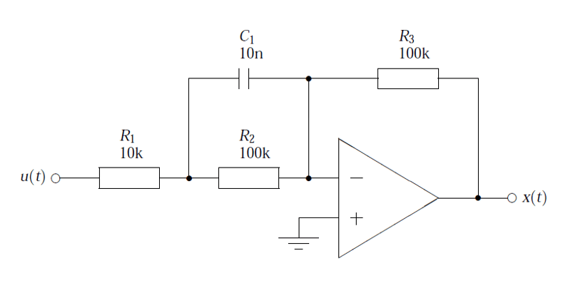
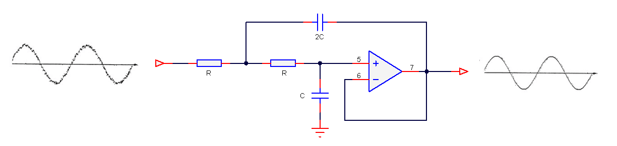
Consider the active pre-emphasis filter shown below. The pre-emphasis filter has found particular use in audio work, since it is necessary to amplify the higher frequencies of the speech spectrum, whilst leaving the lower frequencies unaffected. The R and C values shown are only indented for the example, more practical values will depend on the application. A powerful method of reproducing the magnitude and phases characteristics of the analog filter in a digital implementation, is to mathematically model the circuit. This circuit may be analysed using Kirchhoff’s law, since the sum of currents into the op-amp’s inverting input must be equal to zero for negative feedback to work correctly – this results in a transfer function with a negative gain.
Therefore, using Ohm’s law, i.e. \(I=\frac{V}{R}\),
\(\displaystyle\frac{X(s)}{R_3}=-\frac{U(s)}{C_1||R_2 + R_1}
\)
After some algebraic manipulation, it can be seen that an expression for the circuit’s closed loop gain may be expressed as,
\(\displaystyle\frac{X(s)}{U(s)}=-\frac{R_3}{R_1}\frac{\left(s+\frac{1}{R_2C_1}\right)}{\left(s+\frac{R_1+R_2}{R_1R_2C_1}\right)}
\)
substituting the values shown in the circuit diagram into the developed transfer function, yields
\(\displaystyle H(s)=-10\left(\frac{s+1000}{s+11000}\right)
\)
What sampling rate do we need?
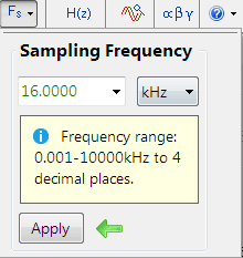
Analysing the cut-off frequencies in \(H(s)\), we see that the upper frequency is at \(11000 rad/sec\) or \(1.75kHz\). Therefore, setting the sampling rate to \(16kHz\) should be adequate for modelling the filter in the digital domain.
The sampling rate options are avaliabe in the main filter design UI (shown on the left).
ASN FilterScript
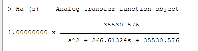
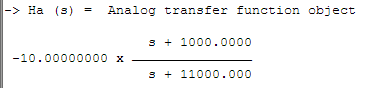
\(H(s)\) can be easily specified in FilterScript with the analogtf function, as follows:
Nb={1,1000};
Na={1,11000};

Ha=analogtf(Nb,Na,-10,"symbolic");
Notice how the negative gain may also be entered directly into function’s argument. The symbolic keyword generates a symbolic transfer function representation in the command window.
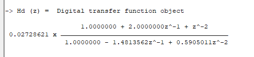
Applying the Bilinear z-transformation via the bilinear command with no pre-warping, i.e.
Hd=bilinear(Ha,0,"symbolic");
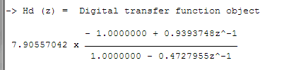
Notice how the bilinear command automatically scales numerator coefficients by -1, in order to account for the effect of the negative gain. The command also automatically assigns the analog filter to the reference spectrum object, which can be shown via the ShowH2DM keyword. The complete code is shown below:
ClearH1;    // remove other filters from the cascade
ShowH2DM;   // show the analog reference spectrum

Main()

Nb={1,1000};
Na={1,11000};

Ha=analogtf(Nb,Na,-10,"symbolic");
Hd=bilinear(Ha,0,"symbolic");

Num=getnum(Hd);
Den=getden(Hd);
Gain=getgain(Hd);
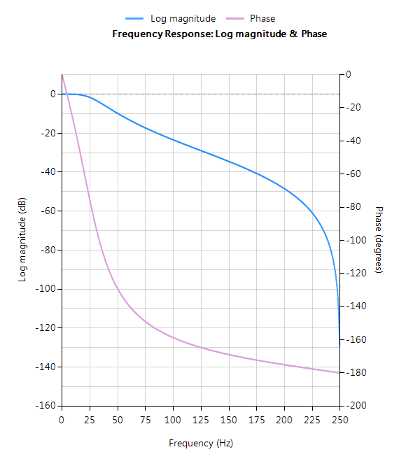
A comparison of the analog (shown in red) and discrete (shown in blue) magnitude spectra is shown below. Analysing the spectra, it can be seen that for a sampling rate of 16kHz the analog and digital filters are almost identical! This demonstrates the relative ease with which a designer can port their existing legacy analog designs into digital.

Automatic code generation to Arm Cortex-M processors
As mentioned at the beginning of this article, the ASN filter designer’s automatic code generation engine facilitates the export of a designed filter to Cortex-M Arm based processor cores via the CMSIS-DSP software framework.
The tool’s built-in analytics and help functions assist the designer in successfully configuring the design for deployment. Professional licence users may expedite the deployment by using the Arm deployment wizard that automates the steps described below.
Steps required for Educational licence users
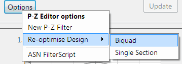
Before generating the code, the H2 filter (i.e. the filter designed in FilterScript) needs to be firstly re-optimised (transformed) to an H1 filter (main filter) structure for deployment. The options menu can be found under the P-Z tab in the main UI.
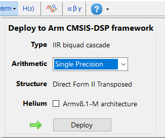
All floating point IIR filters designs must be based on Single Precision arithmetic and either a Direct Form I or Direct Form II Transposed filter structure. The Direct Form II Transposed structure is advocated for floating point implementation by virtue of its higher numerically accuracy.
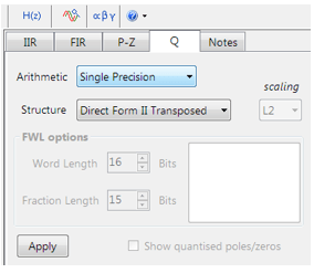
Quantisation and filter structure settings can be found under the Q tab (as shown on the left). Setting Arithmetic to Single Precision and Structure to Direct Form II Transposed and clicking on the Apply button configures the IIR considered herein for the CMSIS-DSP software framework.
Arm CMSIS-DSP application C code
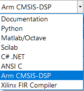
Select the Arm CMSIS-DSP framework from the selection box in the filter summary window:
The automatically generated C code based on the CMSIS-DSP framework for direct implementation on an Arm based Cortex-M processor is shown below:
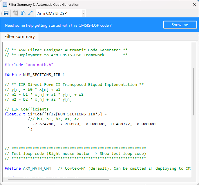
As seen, the automatic code generator generates all initialisation code, scaling and data structures needed to implement the IIR via the CMSIS-DSP library. This code may be directly used in any Cortex-M based development project – a complete Keil MDK example is available on Arm/Keil’s website. Notice that the tool’s code generator produces code for the Cortex-M4 core as default, please refer to the table below for the #define definition required for all supported cores.
ARM_MATH_CM0 | Cortex-M0 core. | ARM_MATH_CM4 | Cortex-M4 core. |
ARM_MATH_CM0PLUS | Cortex-M0+ core. | ARM_MATH_CM7 | Cortex-M7 core. |
ARM_MATH_CM3 | Cortex-M3 core. | ||
ARM_MATH_ARMV8MBL | ARMv8M Baseline target (Cortex-M23 core). | ||
ARM_MATH_ARMV8MML | ARMv8M Mainline target (Cortex-M33 core). |
The main test loop code (not shown) centres around the arm_biquad_cascade_df2T_f32() function, which performs the filtering operation on a block of input data.
What have we learned?
The ASN Filter Designer provides engineers with everything they need in order to port legacy analog filter designs to a variety of Cortex-M processor cores.
The FilterScript symbolic math scripting language offers designers the ability to take an existing analog filter transfer function and transform it to digital (via the Bilinear z-transform or matched z-transform) with just a few lines of code.
The Arm automatic code generator analyses the designed digital filter and then automatically generates Arm CMSIS-DSP compliant C code suitable for direct implementation on a Cortex-M based microcontroller.
Extra resources
- Step by step video tutorial of designing an IIR and deploying it to Keil MDK uVision.
- Implementing Biquad IIR filters with the ASN Filter Designer and the Arm CMSIS-DSP software framework (ASN-AN025)
- Keil MDK uVision example IIR filter project