Modern embedded processors, software frameworks and design tooling now allow engineers to apply advanced measurement concepts to smart factories as part of the I4.0 revolution.
In recent years, PM (predictive maintenance) of machines has received great attention, as factories look to maximise their production efficiency while at the same time retaining the invaluable skills of experienced foremen and production workers.
Traditionally, a foreman would walk around the shop floor and listen to the sounds a machine would make to get an idea of impending failure. With the advent of I4.0 AIoT technology, microphones, edge DSP algorithms and ML may now be employed in order to ‘listen’ to the sounds a machine makes and then make a classification and prediction.
One of the major challenges is how to make a computer hear like a human. In this article we will discuss how sound weighting curves can make a computer hear like a human, and how they can be deployed to an Arm Cortex-M microcontroller for use in an AIoT application.
Physics of the human ear
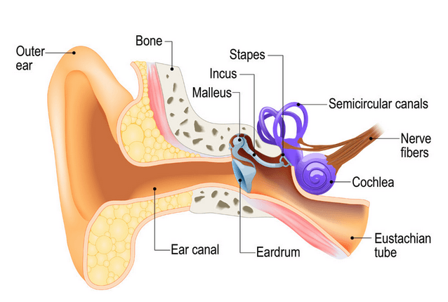
An illustration of the human ear shown below. As seen, the basic task of the ear is to translate sound (air vibration) into electrical nerve impulses for the brain to interpret.
The ear achieves this via three bones (Stapes, Incus and Malleus) that act as a mechanical amplifier for vibrations received at the eardrum. These amplified sounds are then passed onto the Cochlea via the Oval window (not shown).
The Cochlea (shown in purple) is filled with a fluid that moves in response to the vibrations from the oval window. As the fluid moves, thousands of nerve endings are set into motion. These nerve endings transform sound vibrations into electrical impulses that travel along the auditory nerve fibres to the brain for analysis.
Modelling perceived sound
Due to complexity of the fluidic mechanical construction of the human auditory system, low and high frequencies are typically not discernible. Researchers over the years have found that humans are most perceptive to sounds in the 1-6kHz range, although this range varies according to the subject’s physical health.
This research led to the definition of a set of weighting curves: the so-called A, B, C and D weighting curves, which equalises a microphone’s frequency response. These weighting curves aim to bring the digital and physical worlds closer together by allowing a computerised microphone-based system to hear like a human.
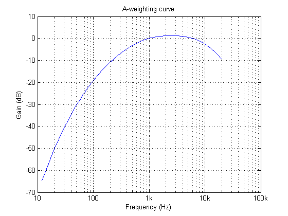
The A-weighing curve is the most widely used as it is mandated by IEC-61672 to be fitted to all sound level meters. The B and D curves are hardly ever used, but C-weighting may be used for testing the impact of noise in telecoms systems.
The frequency response of the A-weighting curve is shown above, where it can be seen that sounds entering our ears are de-emphasised below 500Hz and are most perceptible between 0.5-6kHz. Notice that the curve is unspecified above 20kHz, as this exceeds the human hearing range.
ASN FilterScript
ASN’s FilterScript symbolic math scripting language offers designers the ability to take an analog filter transfer function and transform it to its digital equivalent with just a few lines of code.
The analog transfer functions of the A and C-weighting curves are given below:
\(H_A(s) \approx \displaystyle{7.39705×10^9 \cdot s^4 \over (s + 129.4)^2\quad(s + 676.7)\quad (s + 4636)\quad (s + 76655)^2}\)
\(H_C(s) \approx \displaystyle{5.91797×10^9 \cdot s^2\over(s + 129.4)^2\quad (s + 76655)^2}\)
These analog transfer functions may be transformed into their digital equivalents via the bilinear() function. However, notice that \(H_A(s) \) requires a significant amount of algebracic manipulation in order to extract the denominator cofficients in powers of \(s\).
Convolution
A simple trick to perform polynomial multiplication is to use linear convolution, which is the same algebraic operation as multiplying two polynomials together. This may be easily performed via FilterScript’s conv() function, as follows:
y=conv(a,b);
As a simple example, the multiplication of \((s^2+2s+10)\) with \((s+5)\), would be defined as the following three lines of FilterScript code:
a={1,2,10};
b={1,5};
y=conv(a,b);
which yields, 1 7 20 50 or \((s^3+7s^2+20s+50)\)
For the A-weighting curve Laplace transfer function, the complete FilterScript code is given below:
ClearH1;  // clear primary filter from cascade

Main() // main loop

a={1, 129.4};
b={1, 676.7};
c={1, 4636};
d={1, 76655};

aa=conv(a,a); // polynomial multiplication
dd=conv(d,d);

aab=conv(aa,b);
aabc=conv(aab,c);

Na=conv(aabc,dd);
Nb = {0 ,0 , 1 ,0 ,0 , 0, 0}; // define numerator coefficients
G = 7.397e+09; // define gain

Ha = analogtf(Nb, Na, G, "symbolic");
Hd = bilinear(Ha,0, "symbolic");

Num = getnum(Hd);
Den = getden(Hd);
Gain = getgain(Hd)/computegain(Hd,1e3);    // set gain to 0dB@1kHz
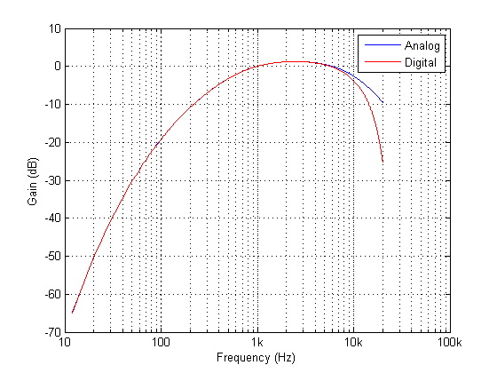
Frequency response of analog vs digital A-weighting filter for \(f_s=48kHz\). As seen, the digital equivalent magnitude response matches the ideal analog magnitude response very closely until \(6kHz\).
The ITU-R 486–4 weighting curve
Another weighting curve of interest is the ITU-R 486–4 weighting curve, developed by the BBC. Unlike the A-weighting filter, the ITU-R 468–4 curve describes subjective loudness for broadband stimuli. The main disadvantage of the A-weighting curve is that it underestimates the loudness judgement of real-world stimuli particularly in the frequency band from about 1–9 kHz.
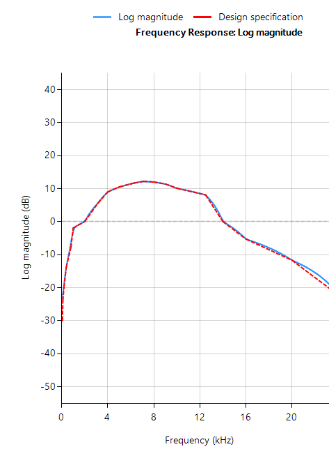
Due to the precise definition of the 486–4 weighting curve, there is no analog transfer function available. Instead the standard provides a table of amplitudes and frequencies – see here. This specification may be directly entered into FilterScript’s firarb() function for designing a suitable FIR filter, as shown below:
Frequency response of an ITU-R 468-4 FIR filter designed with FilterScript’s firarb() function for \(f_s=48kHz\)
As seen, FilterScript provides the designer with a very powerful symbolic scripting language for designing weighting curve filters. The following discussion now focuses on deployment of the A-weighting filter to an Arm based processor via the tool’s automatic code generator. The concepts and steps demonstrated below are equally valid for FIR filters.
Automatic code generation to Arm processor cores via CMSIS-DSP
The ASN Filter Designer’s automatic code generation engine facilitates the export of a designed filter to Cortex-M Arm based processors via the CMSIS-DSP software framework.
The tool’s built-in analytics and help functions assist the designer in successfully configuring the design for deployment. Professional licence users may expedite the deployment by using the Arm deployment wizard that automates the steps described below.
Steps required for Educational licenceusersonly
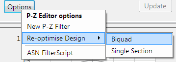
Before generating the code, the H2 filter (i.e. the filter designed in FilterScript) needs to be firstly re-optimised (transformed) to an H1 filter (main filter) structure for deployment. The options menu can be found under the P-Z tab in the main UI.
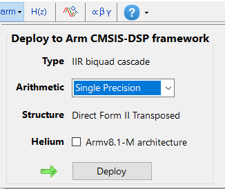
All floating point IIR filters designs must be based on Single Precision arithmetic and either a Direct Form I or Direct Form II Transposed filter structure. The Direct Form II Transposed structure is advocated for floating point implementation by virtue of its higher numerically accuracy.
Quantisation and filter structure settings can be found under the Q tab (as shown on the left). Setting Arithmetic to Single Precision and Structure to Direct Form II Transposed and clicking on the Apply button configures the IIR considered herein for the CMSIS-DSP software framework.
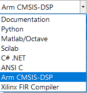
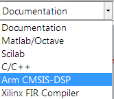
Select the Arm CMSIS-DSP framework from the selection box in the filter summary window:
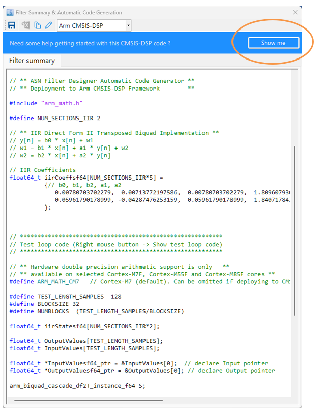
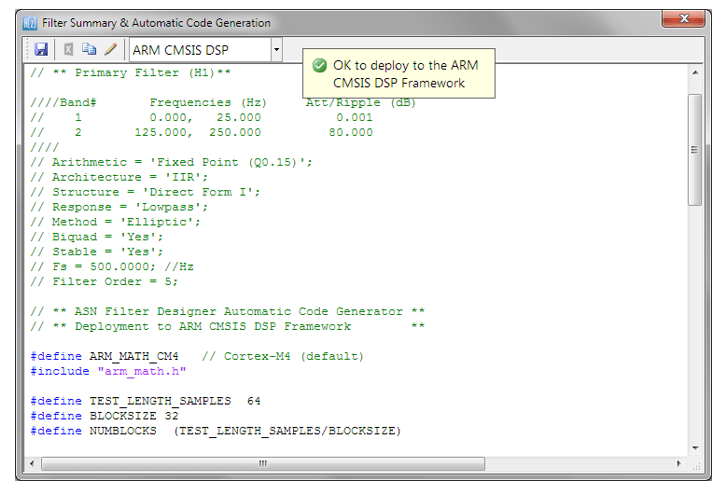
The automatically generated C code based on the CMSIS-DSP framework for direct implementation on an Arm based Cortex-M processor is shown below:
As seen, the ASN Filter Designer’s automatic code generator generates all initialisation code, scaling and data structures needed to implement the A-weighting filter IIR filter via Arm’s CMSIS-DSP library. A detailed help tutorial is available by clicking on the Show me button.
Sanjeev is a RTEI (Real-Time Edge Intelligence) visionary and expert in signals and systems with a track record of successfully developing over 26 commercial products. He is a Distinguished Arm Ambassador and advises top international blue chip companies on their AIoT/RTEI solutions and strategies for I5.0, telemedicine, smart healthcare, smart grids and smart buildings.
https://www.advsolned.com/wp-content/uploads/2019/10/aweightingcurve.png420560Dr. Sanjeev Sarpalhttps://www.advsolned.com/wp-content/uploads/2021/07/asn_logo_red_met_tekst_helder-e1755353934770.pngDr. Sanjeev Sarpal2019-10-03 21:22:482025-06-19 17:00:33A-weighting equalisation: Designing and deploying to Arm Cortex-M microcontrollers
For many IoT sensor measurement applications, an IIR or FIR filter is just one of the many components needed for an algorithm. This could be a powerline interference canceller for a biomedical application or even a simpler DC loadcell filter. In many cases, it is necessary to integrate a filter into a complete algorithm in another domain. ASN Filter Designer’s automatic code generator greatly simlifies exporting to Python.
Python is a very popular general-purpose programming language with support for numerical computing, allowing for the design of algorithms and performing data analysis. The language’s numpy and signal add-on modules attempt to bridge the gap between numerical algorithmic languages, such as Matlab and more traditional programming languages, such as C/C++. As such, it is much more appealing to experienced programmers, who are used to C/C++ data types, syntax and functionality, rather than Matlab’s scripting language that is more aimed at mathematicans developing algorithmic concepts.
ASN Filter Designer automatic code generator for Python
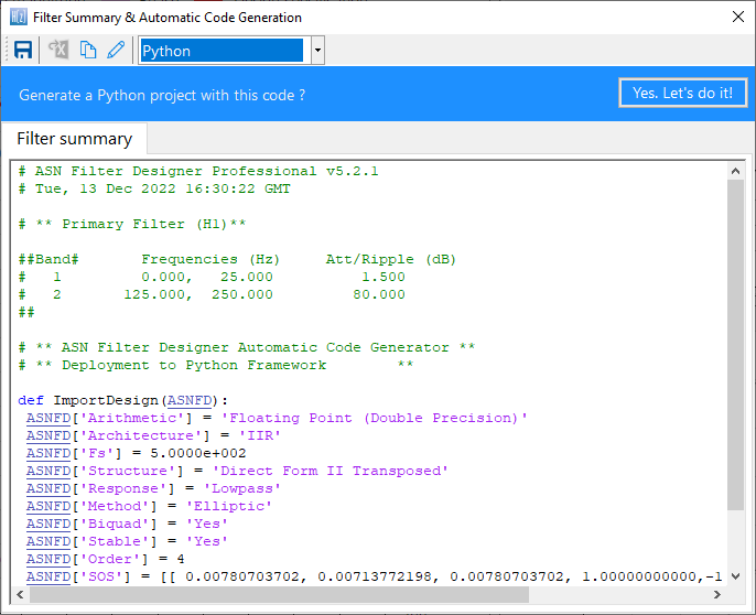
The ASN Filter Designer greatly simplifies exporting a designed filter to Python via its automatic code generator. The code generator supports all aspects of the ASN Filter Designer, allowing for a complete design comprised of H1, H2 and H3 filters and math operators to be fully integrated with an algorithm in Python.
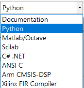
The Python code generator can be accessed via the filter summary options (as shown on the right). Selecting this option will automatically generate a Python .py design file based on the current design settings.
Version 5 of the tool has a completely revamped filter summary UI, and now includes built in AI to analyse the filter cascade for any potential problems.
The project wizard bundles all of the necessary SDK framework files needed to run the designed filter cascade without the need for any other dependencies or 3rd party plugins.
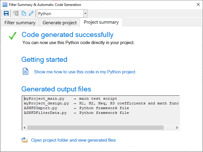
The framework supports both Real and Complex filters in floating point only, and is built on ASN IP blocks, rather than Python’s signal module, which was seen to struggle with managing complex data. Thus, in order to expedite algorithm development with the framework, the following three demos are provided:
ASNFDPythonDemo: main demo file with various examples RMSmeterDemo: An RMS amplitude powerline meter demo EMGDataDemo: An EMG biomedical demo with a HPF, 50Hz notch filter and averaging
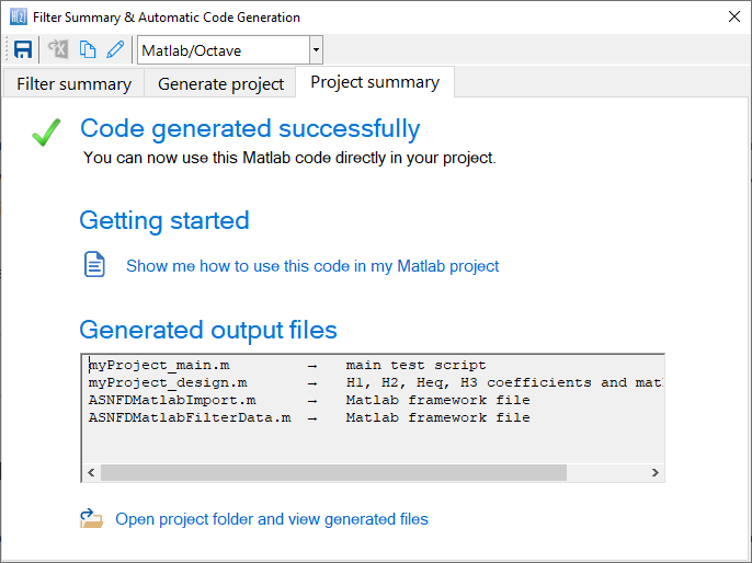
An example of the summary of all of generated files (including the framework files) is shown below.
These files can be used directly in your Python project.
https://www.advsolned.com/wp-content/uploads/2019/01/python-logo.png323666ASN consultancy teamhttps://www.advsolned.com/wp-content/uploads/2021/07/asn_logo_red_met_tekst_helder-e1755353934770.pngASN consultancy team2019-01-08 10:54:102022-12-13 17:25:01How to export designed IIR/FIR filters to Python
IIR (infinite impulse response) filters are generally chosen for applications where linear phase is not too important and memory is limited. They have been widely deployed in audio equalisation, biomedical sensor signal processing, IoT/IIoT smart sensors and high-speed telecommunication/RF applications and form a critical building block in algorithmic design.
Advantages
Low implementation footprint: requires less coefficients and memory than FIR filters in order to satisfy a similar set of specifications, i.e., cut-off frequency and stopband attenuation.
Low latency: suitable for real-time control and very high-speed RF applications by virtue of the low coefficient footprint.
May be used for mimicking the characteristics of analog filters using s-z plane mapping transforms.
Disadvantages
Non-linear phase characteristics.
Requires more scaling and numeric overflow analysis when implemented in fixed point.
Less numerically stable than their FIR (finite impulse response) counterparts, due to the feedback paths.
Definition
An IIR filter is categorised by its theoretically infinite impulse response,
Practically speaking, it is not possible to compute the output of an IIR using this equation. Therefore, the equation may be re-written in terms of a finite number of poles \(p\) and zeros \(q\), as defined by the linear constant coefficient difference equation given by:
where, \(a(k)\) and \(b(k)\) are the filter’s denominator and numerator polynomial coefficients, who’s roots are equal to the filter’s poles and zeros respectively. Thus, a relationship between the difference equation and the z-transform (transfer function) may therefore be defined by using the z-transform delay property such that,
As seen, the transfer function is a frequency domain representation of the filter. Notice also that the poles act on the outputdata, and the zeros on the inputdata. Since the poles act on the output data, and affect stability, it is essential that their radii remain inside the unit circle (i.e. <1) for BIBO (bounded input, bounded output) stability. The radii of the zeros are less critical, as they do not affect filter stability. This is the primary reason why all-zero FIR (finite impulse response) filters are always stable.
A discussion of IIR filter structures for both fixed point and floating point can be found here.
Classical IIR design methods
A discussion of the most commonly used or classical IIR design methods (Butterworth, Chebyshev and Elliptic) will now follow. For anybody looking for more general examples, please visit the ASN blog for the many articles on the subject.
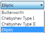
ASN Filter Designer’s graphical designer supports the design of the following four IIR classical design methods:
Butterworth
Chebyshev Type I
Chebyshev Type II
Elliptic
The algorithm used for the computation first designs an analog filter (via an analog design prototype) with the desired filter specifications specified by the graphical design markers – i.e. pass/stopband ripple and cut-off frequencies. The resulting analog filter is then transformed via the Bilinear z-transform into its discrete equivalent for realisation.
Biquad implementations are advocated for numerical stability.
The Bessel prototype is not supported, as the Bilinear transform warps the linear phase characteristics. However, a Bessel filter design method is available in ASN FilterScript.
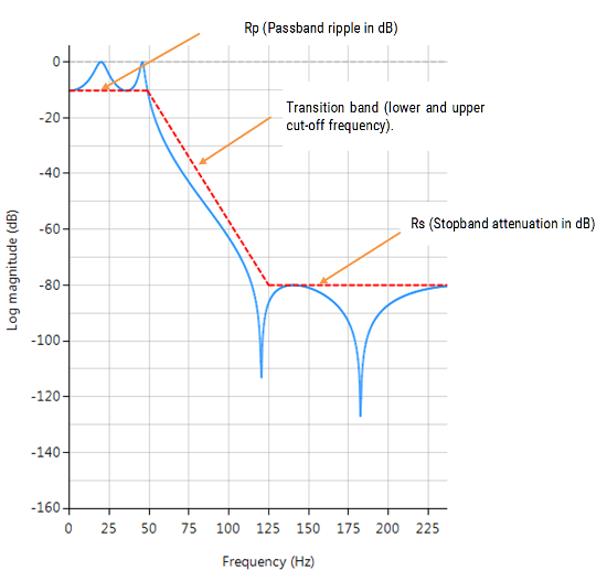
As discussed below, each method has its pros and cons, but in general the Elliptic method should be considered as the first choice as it meets the design specifications with the lowest order of any of the methods. However, this desirable property comes at the expense of ripple in both the passband and stopband, and very non-linear passband phase characteristics. Therefore, the Elliptic filter should only be used in applications where memory is limited and passband phase linearity is less important.
The Butterworth and Chebyshev Type II methods have flat passbands (no ripple), making them a good choice for DC and low frequency measurement applications, such as bridge sensors (e.g. loadcells). However, this desirable property comes at the expense of wider transition bands, resulting in low passband to stopband transition (slow roll-off). The Chebyshev Type I and Elliptic methods roll-off faster but have passband ripple and very non-linear passband phase characteristics.
Comparison of classical design methods
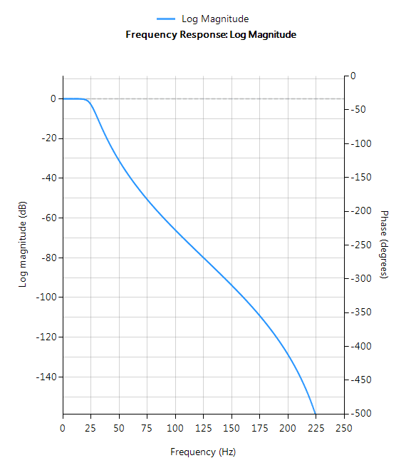
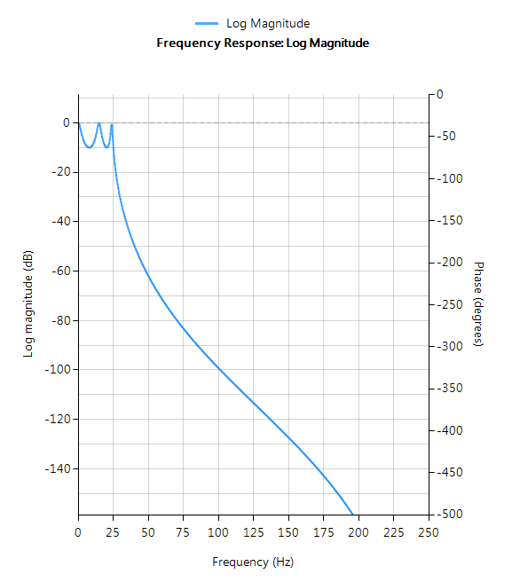
The frequency response charts shown below, show the differences between the various design prototype methods for a 5th order lowpass filter with the same specifications. As seen, the Butterworth response is the slowest to roll-off and the Elliptic the fastest.
Elliptic
Elliptic filters offer steeper roll-off characteristics than Butterworth or Chebyshev filters, but are equiripple in both the passband and the stopband. In general, Elliptic filters meet the design specifications with the lowest order of any of the methods discussed herein.
Filter characteristics
Fastest roll-off of all supported prototypes
Equiripple in both the passband and stopband
Lowest order filter of all supported prototypes
Non-linear passband phase characteristics
Good choice for real-time control and high-throughput (RF applications) applications
Butterworth
Butterworth filters have a magnitude response that is maximally flat in the passband and monotonic overall, making them a good choice for DC and low frequency measurement applications, such as loadcells. However, this highly desirable ‘smoothness’ comes at the price of decreased roll-off steepness. As a consequence, the Butterworth method has the slowest roll-off characteristics of all the methods discussed herein.
Filter characteristics
Smooth monotonic response (no ripple)
Slowest roll-off for equivalent order
Highest order of all supported prototypes
More linear passband phase response than all other methods
Good choice for DC measurement and audio applications
Chebyshev Type I
Chebyshev Type I filters are equiripple in the passband and monotonic in the stopband. As such, Type I filters roll off faster than Chebyshev Type II and Butterworth filters, but at the expense of greater passband ripple.
Filter characteristics
Passband ripple
Maximally flat stopband
Faster roll-off than Butterworth and Chebyshev Type II
Good compromise between Elliptic and Butterworth
Chebyshev Type II
Chebyshev Type II filters are monotonic in the passband and equiripple in the stopband making them a good choice for bridge sensor applications. Although filters designed using the Type II method are slower to roll-off than those designed with the Chebyshev Type I method, the roll-off is faster than those designed with the Butterworth method.
Sanjeev is a RTEI (Real-Time Edge Intelligence) visionary and expert in signals and systems with a track record of successfully developing over 26 commercial products. He is a Distinguished Arm Ambassador and advises top international blue chip companies on their AIoT/RTEI solutions and strategies for I5.0, telemedicine, smart healthcare, smart grids and smart buildings.
For many IoT sensor measurement applications, an IIR or FIR filter is just one of the many components needed for an algorithm. This could be a powerline interference canceller for a biomedical application or even a simpler DC loadcell filter. In many cases, it is necessary to integrate a filter into a complete algorithm in another domain.
Matlab is a well-established numerical computing language developed by the Mathworks that allows for the design of algorithms, matrix data manipulations and data analysis. The product offers a broad range of algorithms and support functions for signal processing applications, and as such is very popular amongst many scientists and engineers worldwide.
ASN Filter Designer automatic code generator for Matlab
The ASN Filter Designer greatly simplifies exporting a designed filter to Matlab via its automatic code generator. The code generator supports all aspects of the ASN Filter Designer, allowing for a complete design comprised of H1, H2 and H3 filters and math operators to be fully integrated with an algorithm in Matlab.
The Matlab code generator can be accessed via the filter summary options (as shown on the right). Selecting this option will automatically generate a Matlab .m file based on the current design.
Version 5 of the tool has a completely revamped filter summary UI, and now includes built in AI to analyse the filter cascade for any potential problems. The project wizard bundles all of the necessary SDK framework files needed to run the designed filter cascade without the need for any other dependencies or 3rd party plugins.
Framework files and examples
In order to use the generated code in Matlab without the need for Signal Processing Toolbox, the following three framework files are provided in the ASN Filter Designer’s \Matlab directory:
These framework files do not have any special Matlab toolbox dependences, and the example script ASNFDMatlabDemo.m demonstrates the simplicity with which the framework can be integrated into your application for your designed filter. Several example filters generated via the automatic code generator are given within ASNFDMatlabDemo.m in order to get you going!
An example of the summary of all of generated files (including the framework files) is shown below.
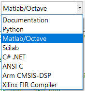
These files can be used directly in your Matlab/Octave project.
Comparing the results to Matlab’s Signal Processing Toolbox
It’s sometimes informative to compare the results of the ASN Filter Designer’s DSP library functions to that of Matlab’s Signal Processing Toolbox.
Designing an IIR Chebyshev Type I filter with the following specifications:
Fs:
500Hz
Passband frequency:
0-25Hz
Type:
Lowpass
Method:
Chebyshev Type I
Stopband attenuation @ 125Hz:
≥ 80 dB
Passband ripple:
≤ 0.1dB
Order:
5
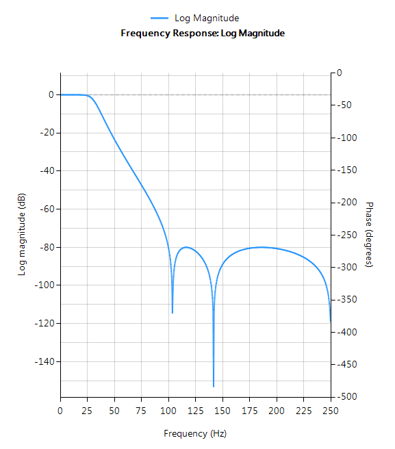
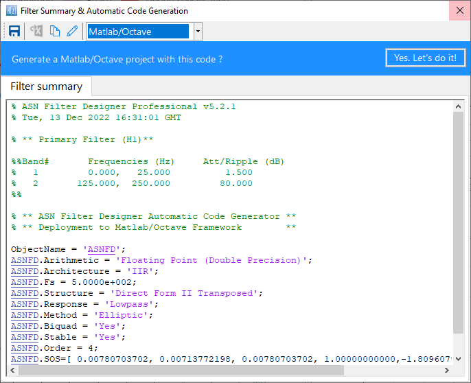
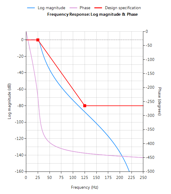
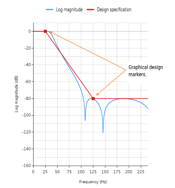
Graphically entering the specifications into the ASN Filter Designer, and fine tuning the design marker positions, the tool automatically designs the filter as a Biquad cascade. Notice that the tool automatically finds the required filter order, and in essence – automatically produces the filter’s exact technical specification!
The frequency response of a 5th order IIR Chebyshev Type I lowpass filter meeting the specifications is shown below:
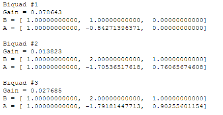
The resulting filter coefficients are:
Designing the same filter in Matlab using Signal Processing Toolbox:
Fs=500;
Rp=0.1;
Rs=80;
F=2*[25,125]/Fs;
[N,Wn]=cheb1ord(F(1),F(2),Rp,Rs)
[z, p, k] = cheby1(N,Rp,Wn,'low'); % design lowpass
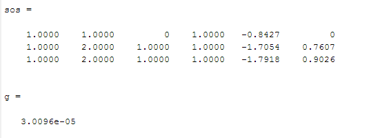
[sos,g]=zp2sos(z,p,k,'up') % generate SOS form
Running the script, we get the following, where each row of sos is a biquad arranged as: b0 b1 b2 a0 a1 a2
Analysing both sets of numerator and denominator coefficients, we get exactly the same result! But what about the gain? Matlab outputs a net gain, g = 3.0096e-05 but the ASN Filter Designer optimally assigns a gain to each biquad. Thus, combining the biquad section gains, i.e. 0.078643, 0.013823 and 0.027685 results in a net gain of 3.0096e-05, which is exactly the same net gain as Matlab!
Conclusion: the ASN Filter Designer’s DSP IIR library functions completely match Matlab’s Signal Processing Toolbox results!!
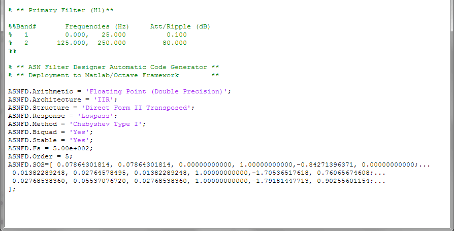
The complete automatically generated code is shown below, where it can be seen that the biquad gains have been pre-multiplied with the feedforward coefficients.
Using the generated code with Signal Processing Toolbox
If you have Signal Processing Toolbox installed, then you may directly use the generated coefficients given in SOS with the sosfilt() command, e.g.
Clear all;

ASNFD_SOS=[ 0.07864301814, 0.07864301814, 0.00000000000, 1.00000000000,-0.84271396371, 0.00000000000;...
 0.01382289248, 0.02764578495, 0.01382289248, 1.00000000000,-1.70536517618, 0.76065674608;...
 0.02768538360, 0.05537076720, 0.02768538360, 1.00000000000,-1.79181447713, 0.90255601154;...
];

y=sosfilt(ASNFD_SOS, x); %  x is your input data

plot(x,y); % plot results
As seen, it is as simple as copying and pasting the filter coefficients from the ASN Filter Designer’s filter summary into a Matlab script.
https://www.advsolned.com/wp-content/uploads/2018/09/matlab.png256256ASN consultancy teamhttps://www.advsolned.com/wp-content/uploads/2021/07/asn_logo_red_met_tekst_helder-e1755353934770.pngASN consultancy team2018-09-25 16:54:072022-12-13 18:12:34How to export designed IIR/FIR filters to Matlab
Infinite impulse response (IIR) filters are useful for a variety of sensor measurement applications, including measurement noise removal and unwanted component cancellation, such as powerline interference. Although several practical implementations for the IIR exist, the Direct form II Transposed structure offers the best numerical accuracy for floating point implementation. However, when considering fixed point implementation on a microcontroller, the Direct Form I structure is considered to be the best choice by virtue of its large accumulator that accommodates any intermediate overflows. This application note specifically addresses IIR biquad filter design and implementation on a Cortex-M based microcontroller with the ASN Filter Designer for both floating point and fixed point applications via the Arm CMSIS-DSP software framework.
Details are also given (including a reference example project) regarding implementation of the IIR filter in Arm/Keil’s MDK industry standard Cortex-M microcontroller development kit.
Introduction
ASN Filter Designer provides engineers with a powerful DSP experimentation platform, allowing for the design, experimentation and deployment of complex IIR and FIR (finite impulse response) digital filter designs for a variety of sensor measurement applications. The tool’s advanced functionality, includes a graphical based real-time filter designer, multiple filter blocks, various mathematical I/O blocks, live symbolic math scripting and real-time signal analysis (via a built-in signal analyser). These advantages coupled with automatic documentation and code generation functionality allow engineers to design and validate a digital filter within minutes rather than hours.
The Arm CMSIS-DSP (Cortex Microcontroller Software Interface Standard) software framework is a rich collection of over sixty DSP functions (including various mathematical functions, such as sine and cosine; IIR/FIR filtering functions, complex math functions, and data types) developed by Arm that have been optimised for their range of Cortex-M processor cores.
The framework makes extensive use of highly optimised SIMD (single instruction, multiple data) instructions, that perform multiple identical operations in a single cycle instruction. The SIMD instructions (if supported by the core) coupled together with other optimisations allow engineers to produce highly optimised signal processing applications for Cortex-M based micro-controllers quickly and simply.
ASN Filter Designer fully supports the CMSIS-DSP software framework, by automatically producing optimised C code based on the framework’s DSP functions via its code generation engine.
Designing IIR filters with the ASN Filter Designer
ASN Filter Designer provides engineers with an easy to use, intuitive graphical design development platform for both IIR and FIR digital filter design. The tool’s real-time design paradigm makes use of graphical design markers, allowing designers to simply draw and modify their magnitude frequency response requirements in real-time while allowing the tool automatically fill in the exact specifications for them.
Consider the design of the following technical specification:
Fs:
500Hz
Passband frequency:
0-40Hz
Type:
Lowpass
Method:
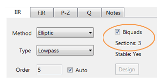
Elliptic
Stopband attenuation @ 125Hz:
≥ 80 dB
Passband ripple:
< 0.1dB
Order:
Small as possible
Graphically entering the specifications into the ASN Filter Designer, and fine tuning the design marker positions, the tool automatically designs the filter as a Biquad cascade (this terminology will be discussed in the following sections), automatically choosing the required filter order, and in essence – automatically producing the filter’s exact technical specification!
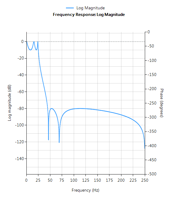
The frequency response of a 5th order IIR Elliptic Lowpass filter meeting the specifications is shown below:
This 5th order Lowpass filter will form the basis of the discussion presented herein.
Biquad IIR filters
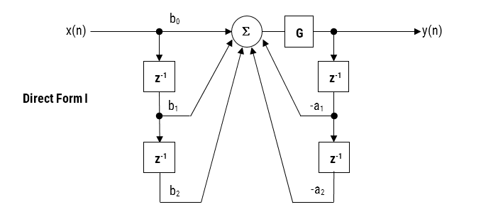
The IIR filter implementation discussed herein is said to be biquad, since it has two poles and two zeros as illustrated below in Figure 1. The biquad implementation is particularly useful for fixed point implementations, as the effects of quantization and numerical stability are minimised. However, the overall success of any biquad implementation is dependent upon the available number precision, which must be sufficient enough in order to ensure that the quantised poles are always inside the unit circle.
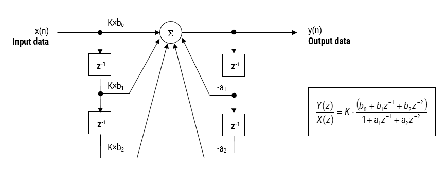
Figure 1: Direct Form I (biquad) IIR filter realization and transfer function.
Analysing Figure 1, it can be seen that the biquad structure is actually comprised of two feedback paths (scaled by \(a_1\) and \(a_2\)), three feed forward paths (scaled by \(b_0, b_1\) and \(b_2\)) and a section gain, \(K\). Thus, the filtering operation of Figure 1 can be summarised by the following simple recursive equation:
Analysing the equation, notice that the biquad implementation only requires four additions (requiring only one accumulator) and five multiplications, which can be easily accommodated on any Cortex-M microcontroller. The section gain, \(K\) may also be pre-multiplied with the forward path coefficients before implementation.
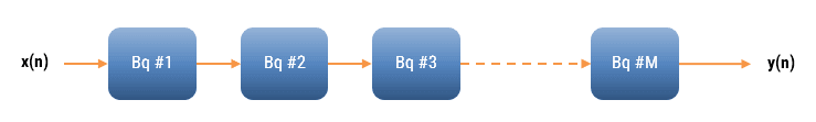
A collection of Biquad filters is referred to as a Biquad Cascade, as illustrated below.
The ASN Filter Designer can design and implement a cascade of up to 50 biquads (Professional edition only).
Floating point implementation
When implementing a filter in floating point (i.e. using double or single precision arithmetic) Direct Form II structures are considered to be a better choice than the Direct Form I structure. The Direct Form II Transposed structure is considered the most numerically accurate for floating point implementation, as the undesirable effects of numerical swamping are minimised as seen by analysing the difference equations.
Figure 2 – Direct Form II Transposed strucutre, transfer function and difference equations
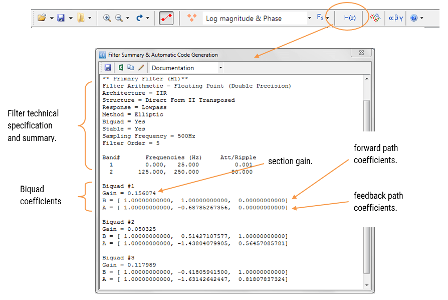
The filter summary (shown in Figure 3) provides the designer with a detailed overview of the designed filter, including a detailed summary of the technical specifications and the filter coefficients, which presents a quick and simple route to documenting your design.
The ASN Filter Designer supports the design and implementation of both single section and Biquad (default setting) IIR filters. However, as the CMSIS-DSP framework does not directly support single section IIR filters, this feature will not be covered in this application note.
The CMSIS-DSP software framework implementation requires sign inversion (i.e. flipping the sign) of the feedback coefficients. In order to accommodate this, the tool’s automatic code generation engine automatically flips the sign of the feedback coefficients as required. In this case, the set of difference equations become,
Automatic code generation to Arm processor cores via CMSIS-DSP
The ASN Filter Designer’s automatic code generation engine facilitates the export of a designed filter to Cortex-M Arm based processors via the CMSIS-DSP software framework. The tool’s built-in analytics and help functions assist the designer in successfully configuring the design for deployment.
All floating point IIR filters designs should be based on Single Precision arithmetic and either a Direct Form I or Direct Form II Transposed filter structure, as this is supported by a hardware multiplier in the M4F, M7F, M33F and M55F cores. Although you may choose Double Precision, hardware support is only available in some M7F and M55F Helium devices. As discussed in the previous section, the Direct Form II Transposed structure is advocated for floating point implementation by virtue of its higher numerically accuracy.
Quantisation and filter structure settings can be found under the Q tab (as shown on the left). Setting Arithmetic to Single Precision and Structure to Direct Form II Transposed and clicking on the Apply button configures the IIR considered herein for the CMSIS-DSP software framework.
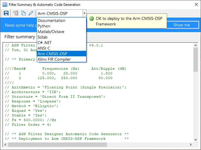
Select the Arm CMSIS-DSP framework from the selection box in the filter summary window:
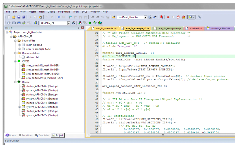
The automatically generated C code based on the CMSIS-DSP framework for direct implementation on an Arm based Cortex-M processor is shown below:
As seen, the automatic code generator generates all initialisation code, scaling and data structures needed to implement the IIR via the CMSIS-DSP library. This code may be directly used in any Cortex-M based development project – a complete Keil MDK example is available on Arm/Keil’s website. Notice that the tool’s code generator produces code for the Cortex-M4 core as default, please refer to the table below for the #define definition required for all supported cores.
ARM_MATH_CM0
Cortex-M0 core.
ARM_MATH_CM4
Cortex-M4 core.
ARM_MATH_CM0PLUS
Cortex-M0+ core.
ARM_MATH_CM7
Cortex-M7 core.
ARM_MATH_CM3
Cortex-M3 core.
ARM_MATH_ARMV8MBL
ARMv8M Baseline target (Cortex-M23 core).
ARM_MATH_ARMV8MML
ARMv8M Mainline target (Cortex-M33 core).
Automatic code generation of complex coefficient IIR filters is currently not supported (see below for more information).
Arm deployment wizard
Professional licence users may expedite the deployment by using the Arm deployment wizard. The built in AI will automatically determine the best settings for your design based on the quantisation settings chosen.
The built in AI automatically analyses your complete filter cascade and converts any H2 or Heq filters into an H1 for implementation. A complex coefficient filter will be automatically converted to real filter for implementation.
Implementing the filter in Arm Keil’s MDK
As mentioned in the previous section, the code generated by the Arm CMSIS-DSP code generator may be directly used in any Cortex-M based development project tooling, such as Arm Keil’s industry standard μVision MDK (microcontroller development kit).
A complete μVision example IIR biquad filter project can be downloaded from Keil’s website, and as seen below is as simple as copying and pasting the code and making minor adjustments to the code.
The example project makes use of μVision’s powerful simulation capabilities, allowing for the evaluation of the IIR filter on M0, M3, M4 and M7 cores respectively. As an added bonus, μVision’s logic analyser may also be used, allowing for comparisons between the ASN Filter Designer’s signal analyser and the reality on a Cortex-M core.
Fixed point implementation
As aforementioned, the Direct Form I filter structure is the best choice for fixed point implementation. However, before implementing the difference equation on a fixed point processor, several important data scaling considerations must be taken into account. As the CMSIS-DSP framework only supports Q15 and Q31 data types for IIR filters, the following discussion relates to an implementation on a 16-bit word architecture, i.e. Q15.
Quantisation
In order to correctly represent the coefficients and input/output numbers, the system word length (16-bit for the purposes of this application note) is first split up into its number of integers and fractional components. The general format is given by:
Q Num of Integers.Fraction length
If we assume that all of data values lie within a maximum/minimum range of \(\pm 1\), we can use Q0.15 format to represent all of the numbers respectively. Notice that Q0.15 (or simply Q15) format represents a maximum of \(\displaystyle 1-2^{-15}=0.9999=0x7FFF\) and a minimum of \(-1=0x8000\) (two’s complement format).
The ASN Filter Designer may be configured for Fixed Point Q15 arithmetic by setting the Word length and Fractional length specifications in the Q Tab (see the configuration section for the details). However, one obvious problem that manifests itself for Biquads is the number range of the coefficients. As poles can be placed anywhere inside the unit circle, the resulting polynomial needed for implementation will often be in the range \(\pm 2\), which would require Q14 arithmetic. In order to overcome this issue, all numerator and denominator coefficients are scaled via a biquad Post Scaling Factor as discussed below.
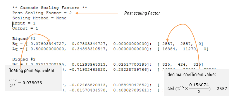
Post Scaling Factor
In order to ensure that coefficients fit within the Word length and Fractional length specifications, all IIR filters include a Post Scaling Factor, which scales the numerator and denominator coefficients accordingly. As a consequence of this scaling, the Post Scaling Factor must be included within the filter structure in order to ensure correct operation.
The Post scaling concept is illustrated below for a Direct Form I biquad implementation.
Figure 4: Direct Form I structure with post scaling.
Pre-multiplying the numerator coefficients with the section gain, \(K\), each coefficient can now be scaled by \(G\), i.e. \(\displaystyle b_0=\frac{b_0}{G}, b_1=\frac{b_1}{G}, a_1=\frac{a_1}{G}, a_2=\frac{a_2}{G}\) and etc. This now results in the following difference equation:
All IIR structures implemented within the tool include the Post Scaling Factor concept. This scaling is mandatory for implementation via the Arm CMSIS-DSP framework – see the configuration section for more details.
Understanding the filter summary
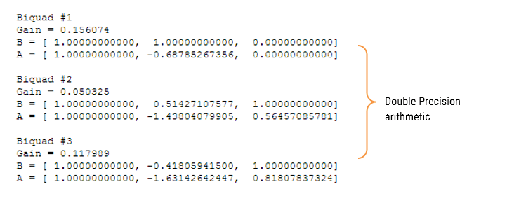
In order to fully understand the information presented in the ASN Filter Designer filter summary, the following example illustrates the filter coefficients obtained with Double Precision arithmetic and with Fixed Point Q15 quantisation.
Applying Fixed Point Q15 arithmetic (note the effects of quantisation on the coefficient values):
Configuring the ASN Filter Designer for Fixed Point arithmetic
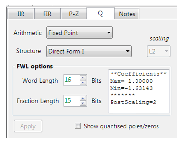
In order to implement an IIR fixed point filter via the CMSIS-DSP framework, all designs must be based on Fixed Point arithmetic (either Q15 or Q31) and the Direct Form I filter structure.
Quantisation and filter structure settings can be found under the Q tab (as shown on the left): Setting Arithmetic to Fixed Point and Structure to Direct Form I and clicking on the Apply button configures the IIR considered herein for the CMSIS-DSP software framework.
The Post Scaling Factor is actually implemented in the CMSIS-DSP software framework as \( \log_2 G\) (i.e. a shift left scaling operation as depicted in Figure 4).
Built in analytics: the tool will automatically analyse the cascade’s filter coefficients and choose an appropriate scaling factor. As seen above, as the largest minimum value is -1.63143, thus, a Post Scaling Factor of 2 is required in order to ‘fit’ all of the coefficients into Q15 arithmetic.
Comparing spectra obtained by different arithmetic rules
In order to improve clarity and overall computation speed, the ASN Filter Designer only displays spectra (i.e. magnitude, phase etc.) based on the current arithmetic rules. This is somewhat different to other tools that display multi-spectra obtained by (for example) Fixed Point and Double Precision arithmetic. For any users wishing to compare spectra you may simply switch between arithmetic settings by changing the Arithmetic method. The designer will then automatically re-compute the filter coefficients using the selected arithmetic rules and the current technical specification. The chart will then be updated using the current zoom settings.
Automatic code generation to the Arm CMSIS-DSP framework
As with floating point arithmetic, select the Arm CMSIS-DSP framework from the selection box in the filter summary window:
The automatically generated C code based on the CMSIS-DSP framework for direct implementation on an Arm based Cortex-M processor is shown below:
As with the floating point filter, the automatic code generator generates all initialisation code, scaling and data structures needed to implement the IIR via the CMSIS-DSP library. This code may be directly used in any Cortex-M based development project – a complete Keil MDK example is available on Arm/Keil’s website. Notice that the tool’s code generator produces code for the Cortex-M4 core as default, please refer to the table below for the #define definition required for all supported cores.
ARM_MATH_CM0
Cortex-M0 core.
ARM_MATH_CM4
Cortex-M4 core.
ARM_MATH_CM0PLUS
Cortex-M0+ core.
ARM_MATH_CM7
Cortex-M7 core.
ARM_MATH_CM3
Cortex-M3 core.
ARM_MATH_ARMV8MBL
ARMv8M Baseline target (Cortex-M23 core).
ARM_MATH_ARMV8MML
ARMv8M Mainline target (Cortex-M33 core).
The main test loop code (not shown) centres around the arm_biquad_cascade_df2T_f32() function, which performs the filtering operation on a block of input data.
Complex coefficient IIR filters are currently not supported.
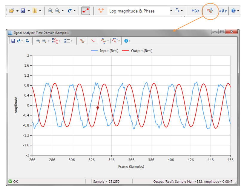
Validating the design with the signal analyser
A design may be validated with the signal analyser, where both time and frequency domain plots are supported. A comprehensive signal generator is fully integrated into the signal analyser allowing designers to test their filters with a variety of input signals, such as sine waves, white noise or even external test data.
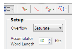
For Fixed Point implementations, the tool allows designers to specify the Overflow arithmetic rules as: Saturate or Wrap. Also, the Accumulator Word Length may be set between 16-40 bits allowing designers to quickly find the optimum settings to suit their application.
Extra resources
Digital signal processing: principles, algorithms and applications, J.Proakis and D.Manoloakis
Digital signal processing: a practical approach, E.Ifeachor and B.Jervis.
Digital filters and signal processing, L.Jackson.
Step by step video tutorial of designing an IIR and deploying it to Keil MDK uVision.
Implementing Biquad IIR filters with the ASN Filter Designer and the Arm CMSIS-DSP software framework (ASN-AN025)
Sanjeev is a RTEI (Real-Time Edge Intelligence) visionary and expert in signals and systems with a track record of successfully developing over 26 commercial products. He is a Distinguished Arm Ambassador and advises top international blue chip companies on their AIoT/RTEI solutions and strategies for I5.0, telemedicine, smart healthcare, smart grids and smart buildings.
https://www.advsolned.com/wp-content/uploads/2018/09/asn25_biquad_postscale.png316678Dr. Sanjeev Sarpalhttps://www.advsolned.com/wp-content/uploads/2021/07/asn_logo_red_met_tekst_helder-e1755353934770.pngDr. Sanjeev Sarpal2018-09-22 22:44:112023-05-12 16:39:11Implementing Biquad IIR filters with the ASN Filter Designer and the Arm CMSIS-DSP software framework