ASN Filter Designer’s new ANSI C SDK framework, provides developers with a comprehensive automatic C code generator for microcontrollers and embedded platforms. This allows developers to directly deploy their AIoT filtering application from within the tool to any STM32, Arduino, ESP32, PIC32, Beagle Bone and other Arm, RISC-V, MIPS microcontrollers for direct use.
Arm’s CMSIS-DSP library vs. ASN’s C SDK Framework
Thanks to our close collaboration with Arm’s architecture team, our new ultra-compact, highly optimised ANSI C based framework provides outstanding performance compared to other commercial DSP libraries, including Arm’s optimised CMSIS-DSP library.
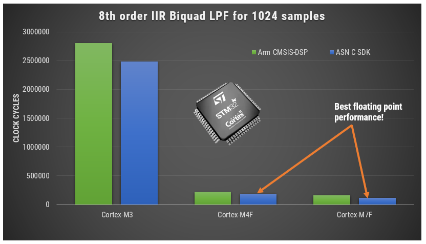
Benchmarks for STM32: M3, M4F and M7F microcontrollers running an 8th order IIR biquad lowpass filter for 1024 samples
As seen, using o1 complier optimisation, our framework is able to surpass Arm’s CMSIS-DSP library’s performance on an M4F and M7F. Although notice that performance of both libraries is worse on the Cortex-M3, as it doesn’t have an FPU. Despite the difference, both libraries perform equally well, but the ASN DSP library has the added advantage of extra functionality and being platform agnostic, making it ideal for variety of biomedical (ECG, EMG, PPG), audio (sound effects, equalisers) , IoT (temperature, gas, pressure) and I4.0 (flow measurement, vibration analysis, CbM) applications.
AIoT applications designed on the newer Cortex-M33F and Cortex-M55F cores can also take advantage of extra filtering blocks, double precision arithmetic support, providing a simple way of implementing high performance AI on the Edge applications within hours.
Advantages for developers
A developer can now develop, test and deploy a complete DSP filtering application within the ASN Filter Designer within a few hours. This is very different from a traditional R&D approach that assigns a team of developers for several days in order to achieve the same level of accuracy required for the application.
Open source and agnostic code base: In order to allow developers to get the maximum performance for their applications, the ASN-DSP SDK is provided as open source and is written in ANSI C. This means that any embedded processor and any level of compiler optimisation can be used.
Memory size required for the ASN-DSP SDK is relativity lower than other standard DSP libraries, which makes the ASN-DSP SDK extremely suitable for microcontrollers that have memory constrains.
Using the ASN Filter Designer’s signal analyser tool, developers now can test the performance, accuracy and assess the frequency response of their designed filter and get optimised C code which they can directly use in their application.
The SDK also supports some extra filtering functions, such as: a median filter, a moving average filter, all-pass, single section IIR filters, a TKEO biomedical filter, and various non-linear functions, including RMS, Abs, Log and Sqrt. These functions form the filter cascade within the tool, and can be used to build signal processing applications, such as EMG and ECG biomedical applications.
The ASN-DSP SDK supports both single and double precision floating point arithmetic, providing excellent numerical accuracy and wide dynamic range. The library is unique in the sense that it supports double precision arithmetic, which although is not the most optimal for microcontrollers, allows for the implementation of high-fidelity filtering applications.
The ANSI C SDK framework is further extended by our new C# .NET framework, allowing .NET developers to build high performance desktop applications with signal processing capabilities.
Find out more and try it yourself
Benchmarks on a variety of 32-bit embedded platforms, including a biomedical EMG filtering example, are covered in the following application note.
The both framework SDKs are available in ASNFD v5.0, which may be downloaded here.
Although the design of FIR filters with linear phase is an easy task. This is certainly not true for IIR filters that usually have a highly non-linear phase response, especially around the filter’s cut-off frequencies. This article discusses the characteristics needed for a digital filter to have linear phase, and how an IIR filter’s passband phase can be modified in order to achieve linear phase using all-pass equalisation filters.
Why do we need linear phase filters?
Digital filters with linear phase have the advantage of delaying all frequency components by the same amount, i.e. they preserve the input signal’s phase relationships. This preservation of phase means that the filtered signal retains the shape of the original input signal. This characteristic is essential for audio applications as the signal shape is paramount for maintaining high fidelity in the filtered audio. Yet another application area that requires this, is ECG biomedical waveform analysis, as any artefacts introduced by the filter may be misinterpreted as heart anomalies.
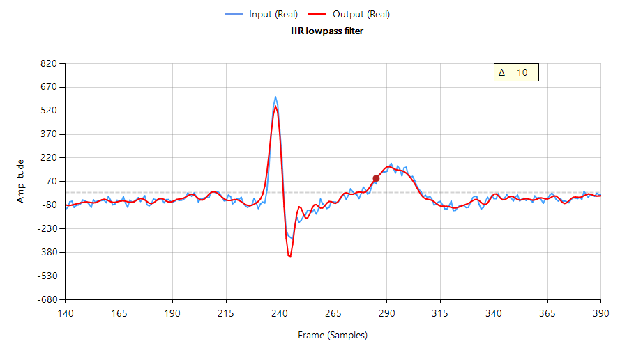
The following plot shows the filtering performance of a Chebyshev type I lowpass IIR on ECG data – input waveform (shown in blue) shifted by 10 samples (\(\small \Delta=10\)) to approximately compensate for the filter’s group delay. Notice that the filtered signal (shown in red) has attenuated, broadened and added oscillations around the ECG peak, which is undesirable.
Figure 1: IIR lowpass filtering result with phase distortion
In order for a digital filter to have linear phase, its impulse response must have conjugate-even or conjugate-odd symmetry about its midpoint. This is readily seen for an FIR filter,
Analysing Eqn. 3, we see that roots (zeros) of \(\small H(z)\) must also be the zeros of \(\small H^\ast (1/z^\ast)\). This means that the roots of \(\small H(z)\) must occur in conjugate reciprocal pairs, i.e. if \(\small z_k\) is a zero of \(\small H(z)\), then \(\small H^\ast (1/z^\ast)\) must also be a zero.
Why IIR filters do not have linear phase
A digital filter is said to be bounded input, bounded output stable, or BIBO stable, if every bounded input gives rise to a bounded output. All IIR filters have either poles or both poles and zeros, and must be BIBO stable, i.e.
Where, \(\small h(k)\) is the filter’s impulse response. Analyzing Eqn. 4, it should be clear that the BIBO stability criterion will only be satisfied if the system’s poles lie inside the unit circle, since the system’s ROC (region of convergence) must include the unit circle. Consequently, it is sufficient to say that a bounded input signal will always produce a bounded output signal if all the poles lie inside the unit circle.
The zeros on the other hand, are not constrained by this requirement, and as a consequence may lie anywhere on z-plane, since they do not directly affect system stability. Therefore, a system stability analysis may be undertaken by firstly calculating the roots of the transfer function (i.e., roots of the numerator and denominator polynomials) and then plotting the corresponding poles and zeros upon the z-plane.
Applying the developed logic to the poles of an IIR filter, we now arrive at a very important conclusion on why IIR filters cannot have linear phase.
A BIBO stable filter must have its poles within the unit circle, and as such in order to get linear phase, an IIR would need conjugate reciprocal poles outside of the unit circle, making it BIBO unstable.
Based upon this statement, it would seem that it’s not possible to design an IIR to have linear phase. However, a discussed below, phase equalisation filters can be used to linearise the passband phase response.
Phase linearisation with all-pass filters
All-pass phase linearisation filters (equalisers) are a well-established method of altering a filter’s phase response while not affecting its magnitude response. A second order (Biquad) all-pass filter is defined as:
Where, \(\small f_c\) is the centre frequency, \(\small r\) is radius of the poles and \(\small f_s\) is the sampling frequency. Notice how the numerator and denominator coefficients are arranged as a mirror image pair of one another. The mirror image property is what gives the all-pass filter its desirable property, namely allowing the designer to alter the phase response while keeping the magnitude response constant or flat over the complete frequency spectrum.
Cascading an APF (all-pass filter) equalisation cascade (comprised of multiple APFs) with an IIR filter, the basic idea is that we only need to linearise the phase response the passband region. The other regions, such as the transition band and stopband may be ignored, as any non-linearities in these regions are of little interest to the overall filtering result.
The challenge
The APF cascade sounds like an ideal compromise for this challenge, but in truth a significant amount of time and very careful fine-tuning of the APF positions is required in order to achieve an acceptable result. Each APF has two variables: \(\small f_c\) and \(\small r\) that need to be optimised, which complicates the solution. This is further complicated by the fact that the more APF stages that are added to the cascade, the higher the overall filter’s group delay (latency) becomes. This latter issue may become problematic for fast real-time closed loop control systems that rely on an IIR’s low latency property.
Nevertheless, despite these challenges, the APF equaliser is a good compromise for linearising an IIRs passband phase characteristics.
The APF equaliser
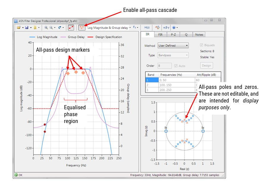
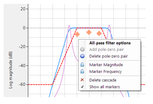
ASN Filter Designer provides designers with a very simple to use graphical all-phase equaliser interface for linearising the passband phase of IIR filters. As seen below, the interface is very intuitive, and allows designers to quickly place and fine-tune APF filters positions with the mouse. The tool automatically calculates \(\small f_c\) and \(\small r\), based on the marker position.
Right clicking on the frequency response chart or on an existing all-pass design marker displays an options menu, as shown on the left.
You may add up to 10 biquads (professional version only).
An IIR with linear passband phase
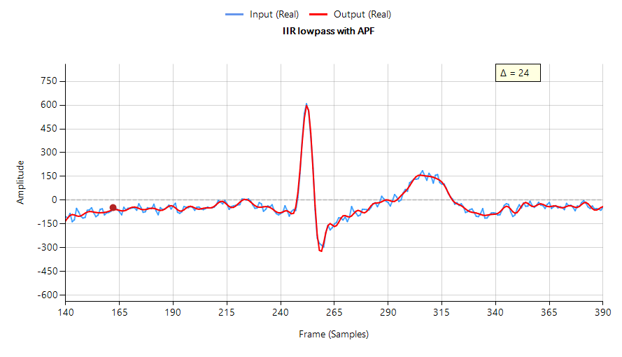
Designing an equaliser composed of three APF pairs, and cascading it with the Chebyshev filter of Figure 1, we obtain a filter waveform that has a much a sharper peak with less attenuation and oscillation than the original IIR – see below. However, this improvement comes at the expense of three extra Biquad filters (the APF cascade) and an increased group delay, which has now risen to 24 samples compared with the original 10 samples.
IIR lowpass filtering result with three APF phase equalisation filters (minimal phase distortion)
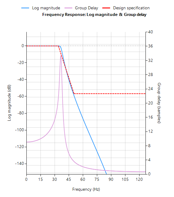
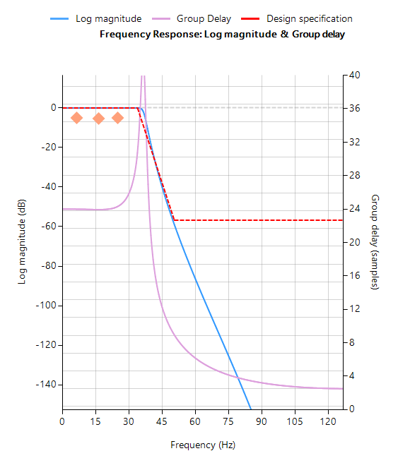
The frequency response of both the original IIR and the equalised IIR are shown below, where the group delay (shown in purple) is the average delay of the filter and is a simpler way of assessing linearity.
IIR without equalisation cascade
IIR with equalisation cascade
Notice that the group delay of the equalised IIR passband (shown on the right) is almost flat, confirming that the phase is indeed linear.
Automatic code generation to Arm processor cores via CMSIS-DSP
The ASN Filter Designer’s automatic code generation engine facilitates the export of a designed filter to Cortex-M Arm based processors via the CMSIS-DSP software framework. The tool’s built-in analytics and help functions assist the designer in successfully configuring the design for deployment.
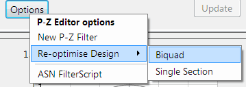
Before generating the code, the IIR and equalisation filters (i.e. H1 and Heq filters) need to be firstly re-optimised (merged) to an H1 filter (main filter) structure for deployment. The options menu can be found under the P-Z tab in the main UI.
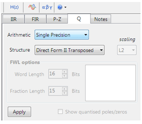
All floating point IIR filters designs should be based on Single Precision arithmetic and either a Direct Form I or Direct Form II Transposed filter structure, as this is supported by a hardware multiplier in the M4F, M7F, M33F and M55F cores. Although you may choose Double Precision, hardware support is only available in some M7F and M55F Helium devices. The Direct Form II Transposed structure is advocated for floating point implementation by virtue of its higher numerically accuracy.
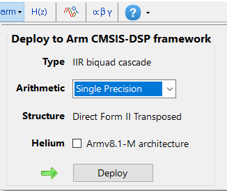
Quantisation and filter structure settings can be found under the Q tab (as shown on the left). Setting Arithmetic to Single Precision and Structure to Direct Form II Transposed and clicking on the Apply button configures the IIR considered herein for the CMSIS-DSP software framework.
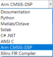
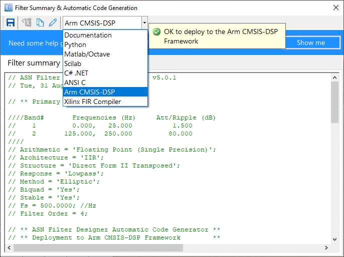
Select the Arm CMSIS-DSP framework from the selection box in the filter summary window:
The automatically generated C code based on the CMSIS-DSP framework for direct implementation on an Arm based Cortex-M processor is shown below:
The ASN Filter Designer’s automatic code generator generates all initialisation code, scaling and data structures needed to implement the linearised filter IIR filter via Arm’s CMSIS-DSP library.
Arm deployment wizard
Professional licence users may expedite the deployment by using the Arm deployment wizard. The built in AI will automatically determine the best settings for your design based on the quantisation settings chosen.
The built in AI automatically analyses your complete filter cascade and converts any H2 or Heq filters into an H1 for implementation.
What we have learnt
The roots of a linear phase digital filter must occur in conjugate reciprocal pairs. Although this no problem for an FIR filter, it becomes infeasible for an IIR filter, as poles would need to be both inside and outside of the unit circle, making the filter BIBO unstable.
The passband phase response of an IIR filter may be linearised by using an APF equalisation cascade. The ASN Filter Designer provides designers with everything they need via a very simple to use, graphical all-pass phase equaliser interface, in order to design a suitable APF cascade by just using the mouse!
The linearised IIR filter may be exported via the automatic code generator using Arm’s optimised CMSIS-DSP library functions for deployment on any Cortex-M microcontroller.
Sanjeev is a RTEI (Real-Time Edge Intelligence) visionary and expert in signals and systems with a track record of successfully developing over 26 commercial products. He is a Distinguished Arm Ambassador and advises top international blue chip companies on their AIoT/RTEI solutions and strategies for I5.0, telemedicine, smart healthcare, smart grids and smart buildings.
A digital filter is a mathematical algorithm that operates on a digital dataset (e.g. sensor data) in order extract information of interest and remove any unwanted information. Applications of this type of technology, include removing glitches from sensor data or even cleaning up noise on a measured signal for easier data analysis. But how do we choose the best type of digital filter for our application? And what are the differences between an IIR filter and an FIR filter?
Digital filters are divided into the following two categories:
Infinite impulse response (IIR)
Finite impulse response (FIR)
As the names suggest, each type of filter is categorised by the length of its impulse response. However, before beginning with a detailed mathematical analysis, it is prudent to appreciate the differences in performance and characteristics of each type of filter.
Example
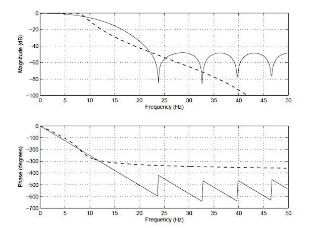
In order to illustrate the differences between an IIR and FIR, the frequency response of a 14th order FIR (solid line), and a 4th order Chebyshev Type I IIR (dashed line) is shown below in Figure 1. Notice that although the magnitude spectra have a similar degree of attenuation, the phase spectrum of the IIR filter is non-linear in the passband (\(\small 0\rightarrow7.5Hz\)), and becomes very non-linear at the cut-off frequency, \(\small f_c=7.5Hz\). Also notice that the FIR requires a higher number of coefficients (15 vs the IIR’s 10) to match the attenuation characteristics of the IIR.
Figure 1:FIR vs IIR: frequency response of a 14th order FIR (solid line), and a 4th order Chebyshev Type I IIR (dashed line)
These are just some of the differences between the two types of filters. A detailed summary of the main advantages and disadvantages of each type of filter will now follow.
IIR filters
IIR (infinite impulse response) filters are generally chosen for applications where linear phase is not too important and memory is limited. They have been widely deployed in audio equalisation, biomedical sensor signal processing, IoT/IIoT smart sensors and high-speed telecommunication/RF applications.
Advantages
Low implementation cost: requires less coefficients and memory than FIR filters in order to satisfy a similar set of specifications, i.e., cut-off frequency and stopband attenuation.
Low latency: suitable for real-time control and very high-speed RF applications by virtue of the low number of coefficients.
Analog equivalent: May be used for mimicking the characteristics of analog filters using s-z plane mapping transforms.
Disadvantages
Non-linear phase characteristics: The phase charactersitics of an IIR filter are generally nonlinear, especially near the cut-off frequencies. All-pass equalisation filters can be used in order to improve the passband phase characteristics.
More detailed analysis: Requires more scaling and numeric overflow analysis when implemented in fixed point. The Direct form II filter structure is especially sensitive to the effects of quantisation, and requires special care during the design phase.
Numerical stability: Less numerically stable than their FIR (finite impulse response) counterparts, due to the feedback paths.
FIR filters
FIR (finite impulse response) filters are generally chosen for applications where linear phase is important and a decent amount of memory and computational performance are available. They have a widely deployed in audio and biomedical signal enhancement applications. Their all-zero structure (discussed below) ensures that they never become unstable for any type of input signal, which gives them a distinct advantage over the IIR.
Advantages
Linear phase: FIRs can be easily designed to have linear phase. This means that no phase distortion is introduced into the signal to be filtered, as all frequencies are shifted in time by the same amount – thus maintaining their relative harmonic relationships (i.e. constant group and phase delay). This is certainly not case with IIR filters, that have a non-linear phase characteristic.
Stability: As FIRs do not use previous output values to compute their present output, i.e. they have no feedback, they can never become unstable for any type of input signal, which is gives them a distinct advantage over IIR filters.
Arbitrary frequency response: The Parks-McClellan and ASN FilterScript’s firarb() function allow for the design of an FIR with an arbitrary magnitude response. This means that an FIR can be customised more easily than an IIR.
Fixed point performance: the effects of quantisation are less severe than that of an IIR.
Disadvantages
High computational and memory requirement: FIRs usually require many more coefficients for achieving a sharp cut-off than their IIR counterparts. The consequence of this is that they require much more memory and significantly a higher amount of MAC (multiple and accumulate) operations. However, modern microcontroller architectures based on the Arm’s Cortex-M cores now include DSP hardware support via SIMD (signal instruction, multiple data) that expedite the filtering operation significantly.
Higher latency: the higher number of coefficients, means that in general a linear phase FIR is less suitable than an IIR for fast high throughput applications. This becomes problematic for real-time closed-loop control applications, where a linear phase FIR filter may have too much group delay to achieve loop stability.
Minimum phase filters: A solution to ovecome the inherent N/2 latency (group delay) in a linear filter is to use a so-called minimum phase filter, whereby any zeros outside of the unit circle are moved to their conjugate reciprocal locations inside the unit circle. The result of thezero flipping operation is that the magnitude spectrum will be identical to the original filter, and the phase will be nonlinear, but most importantly the latency will be reduced from N/2 to something much smaller (although non-constant), making it suitable for real-time control applications. For applications where phase is less important, this may sound ideal, but the difficulty arises in the numerical accuracy of the root-finding algorithm when dealing with large polynomials. Therefore, orders of 50 or 60 should be considered a maximum when using this approach. Although other methods do exist (e.g. the Complex Cepstrum), transforming higher-order linear phase FIRs to their minimum phase cousins remains a challenging task.
No analog equivalent: using the Bilinear, matched z-transform (s-z mapping), an analog filter can be easily be transformed into an equivalent IIR filter. However, this is not possible for an FIR as it has no analog equivalent.
Mathematical definitions
As discussed in the introduction, the name IIR and FIR originate from the mathematical definitions of each type of filter, i.e. an IIR filter is categorised by its theoretically infinite impulse response,
Practically speaking, it is not possible to compute the output of an IIR using this equation. Therefore, the equation may be re-written in terms of a finite number of poles \(\small p\) and zeros \(\small q\), as defined by the linear constant coefficient difference equation given by:
where, \(\small a_k\) and \(\small b_k\) are the filter’s denominator and numerator polynomial coefficients, who’s roots are equal to the filter’s poles and zeros respectively. Thus, a relationship between the difference equation and the z-transform (transfer function) may therefore be defined by using the z-transform delay property such that,
As seen, the transfer function is a frequency domain representation of the filter. Notice also that the poles act on the outputdata, and the zeros on the inputdata. Since the poles act on the output data, and affect stability, it is essential that their radii remain inside the unit circle (i.e. <1) for BIBO (bounded input, bounded output) stability. The radii of the zeros are less critical, as they do not affect filter stability. This is the primary reason why all-zero FIR (finite impulse response) filters are always stable.
BIBO stability
A linear time invariant (LTI) system (such as a digital filter) is said to be bounded input, bounded output stable, or BIBO stable, if every bounded input gives rise to a bounded output, as
Where, \(\small h(k)\) is the LTI system’s impulse response. Analyzing this equation, it should be clear that the BIBO stability criterion will only be satisfied if the system’s poles lie inside the unit circle, since the system’s ROC (region of convergence) must include the unit circle. Consequently, it is sufficient to say that a bounded input signal will always produce a bounded output signal if all the poles lie inside the unit circle.
The zeros on the other hand, are not constrained by this requirement, and as a consequence may lie anywhere on z-plane, since they do not directly affect system stability. Therefore, a system stability analysis may be undertaken by firstly calculating the roots of the transfer function (i.e., roots of the numerator and denominator polynomials) and then plotting the corresponding poles and zeros upon the z-plane.
An interesting situation arises if any poles lie on the unit circle, since the system is said to be marginally stable, as it is neither stable or unstable. Although marginally stable systems are not BIBO stable, they have been exploited by digital oscillator designers, since their impulse response provides a simple method of generating sine waves, which have proved to be invaluable in the field of telecommunications.
Biquad IIR filters
The IIR filter implementation discussed herein is said to be biquad, since it has two poles and two zeros as illustrated below in Figure 2. The biquad implementation is particularly useful for fixed point implementations, as the effects of quantization and numerical stability are minimised. However, the overall success of any biquad implementation is dependent upon the available number precision, which must be sufficient enough in order to ensure that the quantised poles are always inside the unit circle.
Figure 2: Direct Form I (biquad) IIR filter realization and transfer function.
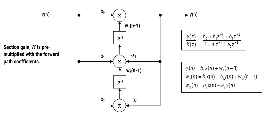
Analysing Figure 2, it can be seen that the biquad structure is actually comprised of two feedback paths (scaled by \(\small a_1\) and \(\small a_2\)), three feed forward paths (scaled by \(\small b_0, b_1\) and \(\small b_2\)) and a section gain, \(\small K\). Thus, the filtering operation of Figure 1 can be summarised by the following simple recursive equation:
Analysing the equation, notice that the biquad implementation only requires four additions (requiring only one accumulator) and five multiplications, which can be easily accommodated on any Cortex-M microcontroller. The section gain, \(\small K\) may also be pre-multiplied with the forward path coefficients before implementation.
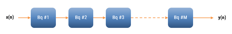
A collection of Biquad filters is referred to as a Biquad Cascade, as illustrated below.
The ASN Filter Designer can design and implement a cascade of up to 50 biquads (Professional edition only).
Floating point implementation
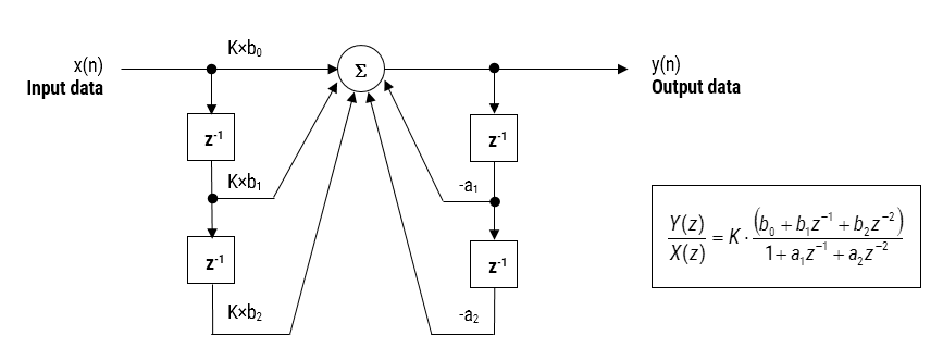
When implementing a filter in floating point (i.e. using double or single precision arithmetic) Direct Form II structures are considered to be a better choice than the Direct Form I structure. The Direct Form II Transposed structure is considered the most numerically accurate for floating point implementation, as the undesirable effects of numerical swamping are minimised as seen by analysing the difference equations.
Figure 3 – Direct Form II Transposed strucutre, transfer function and difference equations
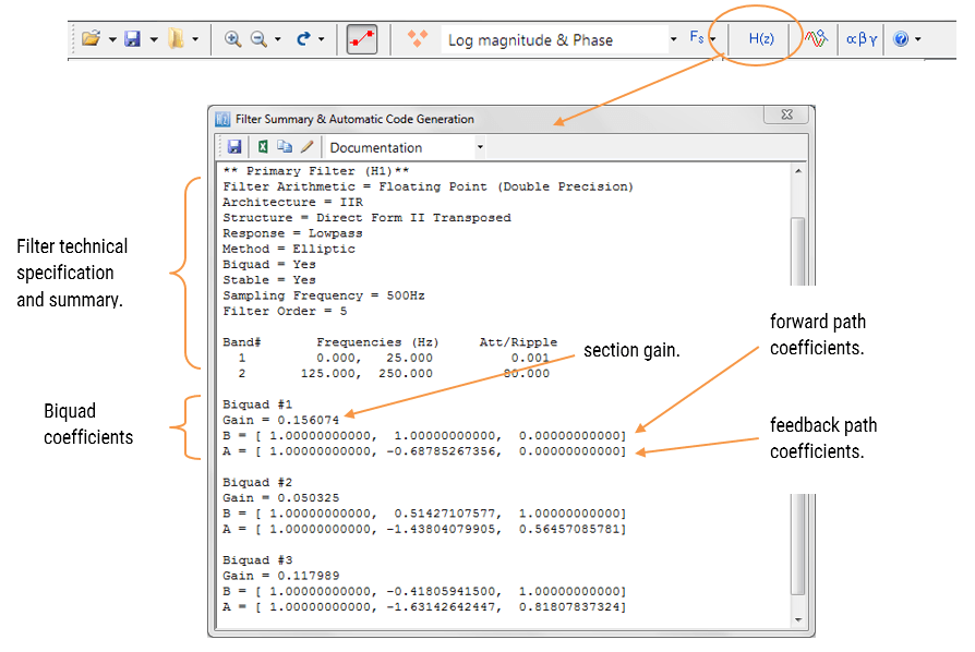
The filter summary (shown in Figure 4) provides the designer with a detailed overview of the designed filter, including a detailed summary of the technical specifications and the filter coefficients, which presents a quick and simple route to documenting your design.
The ASN Filter Designer supports the design and implementation of both single section and Biquad (default setting) IIR filters.
Figure 4: detailed specification.
FIR definition
Returning the IIR’s linear constant coefficient difference equation, i.e.
Notice that when we set the \(\small a_k\) coefficients (i.e. the feedback) to zero, the definition reduces to our original the FIR filter definition, meaning that the FIR computation is just based on past and present inputs values, namely:
\(\displaystyle
y(n)=\sum_{k=0}^{q}b_kx(n-k)
\)
Implementation
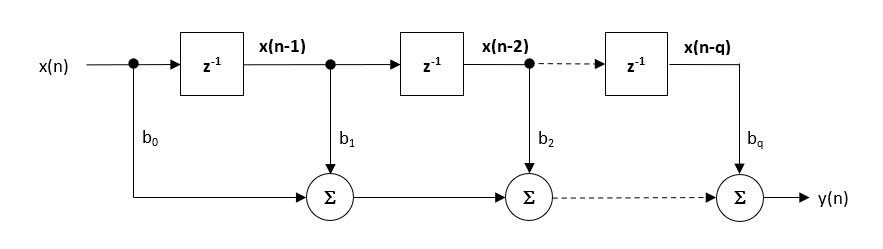
Although several practical implementations for FIRs exist, the direct formstructure and its transposed cousin are perhaps the most commonly used, and as such, all designed filter coefficients are intended for implementation in a Direct form structure.
The Direct form structure and associated difference equation are shown below. The Direct Form is advocated for fixed point implementation by virtue of the single accumulator concept.
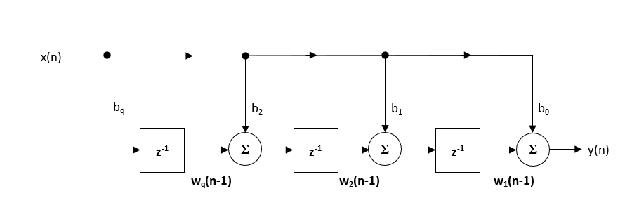
The recommended (default) structure within the ASN Filter Designer is the Direct Form Transposed structure, as this offers superior numerical accuracy when using floating point arithmetic. This can be readily seen by analysing the difference equations below (used for implementation), as the undesirable effects of numerical swamping are minimised, since floating point addition is performed on numbers of similar magnitude.
Implementing your filter on an Arm Cortex-M processor
Although a few processor technologies exist for microcontrollers (e.g. RISC-V, Xtensa, MIPS), over 90% of the microcontrollers used in the smart product market are powered by so-called Arm Cortex-M processors that offer a combination of high algorithmic performance, low-power and security. The Arm Cortex-M4 is a very popular choice with several silicon vendors (including ST, TI, NXP, ADI, Nordic, Microchip, Renesas), as it offers DSP (digital signal processing) functionality traditionally found in more expensive devices and is low-power.
Filtering libraries and support
Arm and ASN provide developers with extensive easy-to-use tooling and tried and tested software libraries used internationally by tens of thousands of developers.
The Arm CMSIS-DSP software framework is interesting as it provides IoT developers with a rich collection of fast mathematical and vector functions, interpolation functions, digital filtering (FIR/IIR) and adaptive filtering (LMS) functions, motor control functions (e.g. PID controller), complex math functions and supports various data types, including fixed and floating point. The important point to make here is that all of these functions have been optimised for Arm Cortex-M processors, allowing you to focus on your application rather than worrying about optimisation.
Despite the broad functionality, the CMSIS-DSP library is somewhat limited for filters, so the flexible ASN DSP filtering library can be used instead, which supports the higher numerical accuracy Direct Form Transposed FIR filter structure and single section IIR filters. A benchmark of ASN’s floating point application-specific DSP filtering library versus Arm’s CMSIS-DSP library is shown below for three types of Arm cores.
Framework Benchmarks: lower number of clock cycles means higher performance.
As seen, the performance of the ASN library is slightly faster by virtue of the application-specific nature of the implementation. The C code is automatically generated from the ASN Filter Designer tool.
What have we learned?
Digital filters are divided into the following two categories:
Infinite impulse response (IIR)
Finite impulse response (FIR)
IIR (infinite impulse response) filters are generally chosen for applications where linear phase is not too important and memory is limited. They have been widely deployed in audio equalisation, biomedical sensor signal processing, IoT/AIoT smart sensors and high-speed telecommunication/RF applications.
FIR (finite impulse response) filters are generally chosen for applications where linear phase is important and a decent amount of memory and computational performance are available. They have a widely deployed in audio and biomedical signal enhancement applications.
ASN Filter Designer provides engineers with everything they need to design, experiment and deploy complex IIR and FIR digital filters for a variety of IoT sensor measurement applications. These advantages coupled with automatic C code generation with ASN’s DSP filtering library functionality allow engineers to design, validate and then deploy their designs to an Arm Cortex-M processor within hours rather than more traditional routes that could take days.
Sanjeev is a RTEI (Real-Time Edge Intelligence) visionary and expert in signals and systems with a track record of successfully developing over 26 commercial products. He is a Distinguished Arm Ambassador and advises top international blue chip companies on their AIoT/RTEI solutions and strategies for I5.0, telemedicine, smart healthcare, smart grids and smart buildings.
https://www.advsolned.com/wp-content/uploads/2020/04/fir_iir.png453622Dr. Sanjeev Sarpalhttps://www.advsolned.com/wp-content/uploads/2021/07/asn_logo_red_met_tekst_helder-e1755353934770.pngDr. Sanjeev Sarpal2020-04-28 13:35:442024-12-05 11:32:35Difference between IIR and FIR filters: a practical design guide
IIR (infinite impulse response) filters are generally chosen for applications where linear phase is not too important and memory is limited. They have been widely deployed in audio equalisation, biomedical sensor signal processing, IoT/IIoT smart sensors and high-speed telecommunication/RF applications and form a critical building block in algorithmic design.
Advantages
Low implementation footprint: requires less coefficients and memory than FIR filters in order to satisfy a similar set of specifications, i.e., cut-off frequency and stopband attenuation.
Low latency: suitable for real-time control and very high-speed RF applications by virtue of the low coefficient footprint.
May be used for mimicking the characteristics of analog filters using s-z plane mapping transforms.
Disadvantages
Non-linear phase characteristics.
Requires more scaling and numeric overflow analysis when implemented in fixed point.
Less numerically stable than their FIR (finite impulse response) counterparts, due to the feedback paths.
Definition
An IIR filter is categorised by its theoretically infinite impulse response,
Practically speaking, it is not possible to compute the output of an IIR using this equation. Therefore, the equation may be re-written in terms of a finite number of poles \(p\) and zeros \(q\), as defined by the linear constant coefficient difference equation given by:
where, \(a(k)\) and \(b(k)\) are the filter’s denominator and numerator polynomial coefficients, who’s roots are equal to the filter’s poles and zeros respectively. Thus, a relationship between the difference equation and the z-transform (transfer function) may therefore be defined by using the z-transform delay property such that,
As seen, the transfer function is a frequency domain representation of the filter. Notice also that the poles act on the outputdata, and the zeros on the inputdata. Since the poles act on the output data, and affect stability, it is essential that their radii remain inside the unit circle (i.e. <1) for BIBO (bounded input, bounded output) stability. The radii of the zeros are less critical, as they do not affect filter stability. This is the primary reason why all-zero FIR (finite impulse response) filters are always stable.
A discussion of IIR filter structures for both fixed point and floating point can be found here.
Classical IIR design methods
A discussion of the most commonly used or classical IIR design methods (Butterworth, Chebyshev and Elliptic) will now follow. For anybody looking for more general examples, please visit the ASN blog for the many articles on the subject.
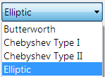
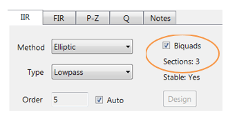
ASN Filter Designer’s graphical designer supports the design of the following four IIR classical design methods:
Butterworth
Chebyshev Type I
Chebyshev Type II
Elliptic
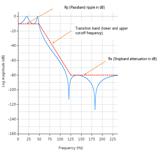
The algorithm used for the computation first designs an analog filter (via an analog design prototype) with the desired filter specifications specified by the graphical design markers – i.e. pass/stopband ripple and cut-off frequencies. The resulting analog filter is then transformed via the Bilinear z-transform into its discrete equivalent for realisation.
Biquad implementations are advocated for numerical stability.
The Bessel prototype is not supported, as the Bilinear transform warps the linear phase characteristics. However, a Bessel filter design method is available in ASN FilterScript.
As discussed below, each method has its pros and cons, but in general the Elliptic method should be considered as the first choice as it meets the design specifications with the lowest order of any of the methods. However, this desirable property comes at the expense of ripple in both the passband and stopband, and very non-linear passband phase characteristics. Therefore, the Elliptic filter should only be used in applications where memory is limited and passband phase linearity is less important.
The Butterworth and Chebyshev Type II methods have flat passbands (no ripple), making them a good choice for DC and low frequency measurement applications, such as bridge sensors (e.g. loadcells). However, this desirable property comes at the expense of wider transition bands, resulting in low passband to stopband transition (slow roll-off). The Chebyshev Type I and Elliptic methods roll-off faster but have passband ripple and very non-linear passband phase characteristics.
Comparison of classical design methods
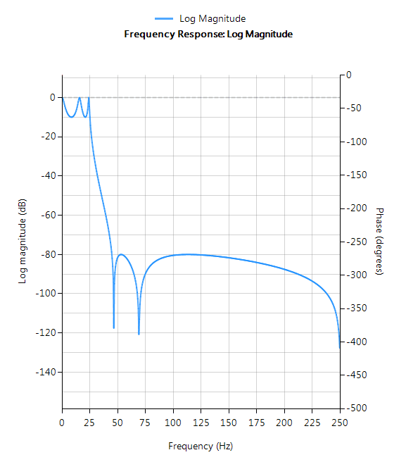
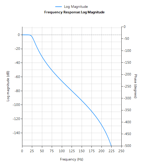
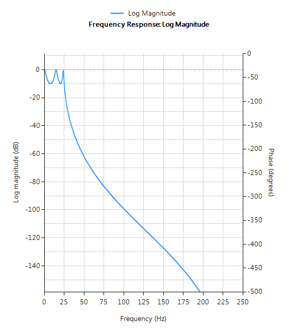
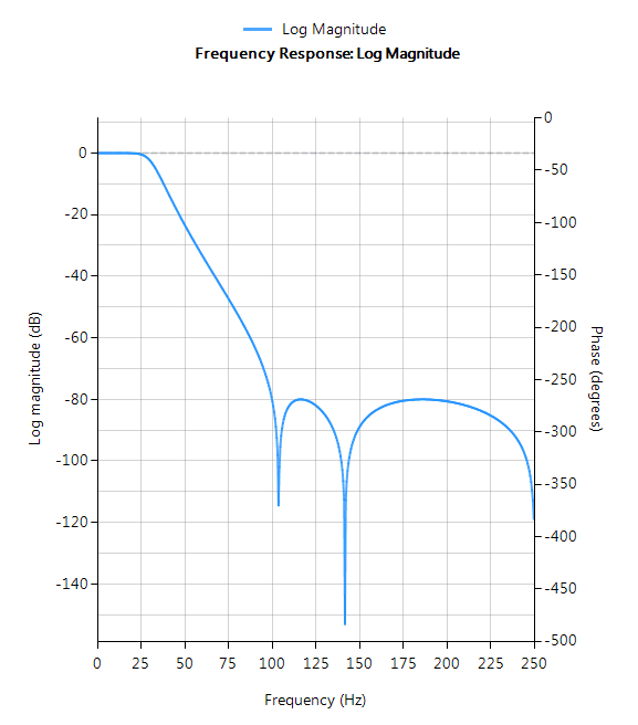
The frequency response charts shown below, show the differences between the various design prototype methods for a 5th order lowpass filter with the same specifications. As seen, the Butterworth response is the slowest to roll-off and the Elliptic the fastest.
Elliptic
Elliptic filters offer steeper roll-off characteristics than Butterworth or Chebyshev filters, but are equiripple in both the passband and the stopband. In general, Elliptic filters meet the design specifications with the lowest order of any of the methods discussed herein.
Filter characteristics
Fastest roll-off of all supported prototypes
Equiripple in both the passband and stopband
Lowest order filter of all supported prototypes
Non-linear passband phase characteristics
Good choice for real-time control and high-throughput (RF applications) applications
Butterworth
Butterworth filters have a magnitude response that is maximally flat in the passband and monotonic overall, making them a good choice for DC and low frequency measurement applications, such as loadcells. However, this highly desirable ‘smoothness’ comes at the price of decreased roll-off steepness. As a consequence, the Butterworth method has the slowest roll-off characteristics of all the methods discussed herein.
Filter characteristics
Smooth monotonic response (no ripple)
Slowest roll-off for equivalent order
Highest order of all supported prototypes
More linear passband phase response than all other methods
Good choice for DC measurement and audio applications
Chebyshev Type I
Chebyshev Type I filters are equiripple in the passband and monotonic in the stopband. As such, Type I filters roll off faster than Chebyshev Type II and Butterworth filters, but at the expense of greater passband ripple.
Filter characteristics
Passband ripple
Maximally flat stopband
Faster roll-off than Butterworth and Chebyshev Type II
Good compromise between Elliptic and Butterworth
Chebyshev Type II
Chebyshev Type II filters are monotonic in the passband and equiripple in the stopband making them a good choice for bridge sensor applications. Although filters designed using the Type II method are slower to roll-off than those designed with the Chebyshev Type I method, the roll-off is faster than those designed with the Butterworth method.
Sanjeev is a RTEI (Real-Time Edge Intelligence) visionary and expert in signals and systems with a track record of successfully developing over 26 commercial products. He is a Distinguished Arm Ambassador and advises top international blue chip companies on their AIoT/RTEI solutions and strategies for I5.0, telemedicine, smart healthcare, smart grids and smart buildings.