IIR (infinite impulse response) filters are generally chosen for applications where linear phase is not too important and memory is limited. They have been widely deployed in audio equalisation, biomedical sensor signal processing, IoT/IIoT smart sensors and high-speed telecommunication/RF applications and form a critical building block in algorithmic design.
Advantages
- Low implementation footprint: requires less coefficients and memory than FIR filters in order to satisfy a similar set of specifications, i.e., cut-off frequency and stopband attenuation.
- Low latency: suitable for real-time control and very high-speed RF applications by virtue of the low coefficient footprint.
- May be used for mimicking the characteristics of analog filters using s-z plane mapping transforms.
Disadvantages
- Non-linear phase characteristics.
- Requires more scaling and numeric overflow analysis when implemented in fixed point.
- Less numerically stable than their FIR (finite impulse response) counterparts, due to the feedback paths.
Definition
An IIR filter is categorised by its theoretically infinite impulse response,
Practically speaking, it is not possible to compute the output of an IIR using this equation. Therefore, the equation may be re-written in terms of a finite number of poles \(p\) and zeros \(q\), as defined by the linear constant coefficient difference equation given by:
where, \(a(k)\) and \(b(k)\) are the filter’s denominator and numerator polynomial coefficients, who’s roots are equal to the filter’s poles and zeros respectively. Thus, a relationship between the difference equation and the z-transform (transfer function) may therefore be defined by using the z-transform delay property such that,
As seen, the transfer function is a frequency domain representation of the filter. Notice also that the poles act on the output data, and the zeros on the input data. Since the poles act on the output data, and affect stability, it is essential that their radii remain inside the unit circle (i.e. <1) for BIBO (bounded input, bounded output) stability. The radii of the zeros are less critical, as they do not affect filter stability. This is the primary reason why all-zero FIR (finite impulse response) filters are always stable.
A discussion of IIR filter structures for both fixed point and floating point can be found here.
Classical IIR design methods
A discussion of the most commonly used or classical IIR design methods (Butterworth, Chebyshev and Elliptic) will now follow. For anybody looking for more general examples, please visit the ASN blog for the many articles on the subject.
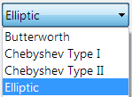
ASN Filter Designer’s graphical designer supports the design of the following four IIR classical design methods:
- Butterworth
- Chebyshev Type I
- Chebyshev Type II
- Elliptic
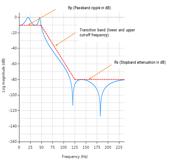
The algorithm used for the computation first designs an analog filter (via an analog design prototype) with the desired filter specifications specified by the graphical design markers – i.e. pass/stopband ripple and cut-off frequencies. The resulting analog filter is then transformed via the Bilinear z-transform into its discrete equivalent for realisation.
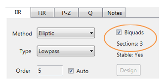

Biquad implementations are advocated for numerical stability.
The Bessel prototype is not supported, as the Bilinear transform warps the linear phase characteristics. However, a Bessel filter design method is available in ASN FilterScript.
As discussed below, each method has its pros and cons, but in general the Elliptic method should be considered as the first choice as it meets the design specifications with the lowest order of any of the methods. However, this desirable property comes at the expense of ripple in both the passband and stopband, and very non-linear passband phase characteristics. Therefore, the Elliptic filter should only be used in applications where memory is limited and passband phase linearity is less important.
The Butterworth and Chebyshev Type II methods have flat passbands (no ripple), making them a good choice for DC and low frequency measurement applications, such as bridge sensors (e.g. loadcells). However, this desirable property comes at the expense of wider transition bands, resulting in low passband to stopband transition (slow roll-off). The Chebyshev Type I and Elliptic methods roll-off faster but have passband ripple and very non-linear passband phase characteristics.
Comparison of classical design methods
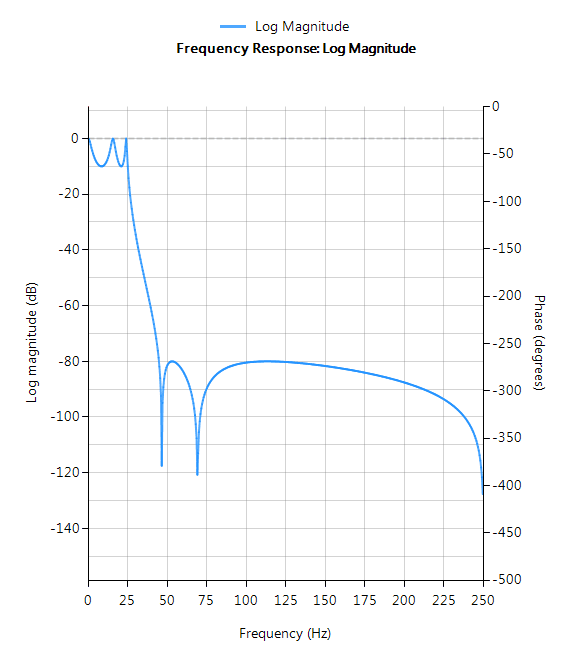
The frequency response charts shown below, show the differences between the various design prototype methods for a 5th order lowpass filter with the same specifications. As seen, the Butterworth response is the slowest to roll-off and the Elliptic the fastest.
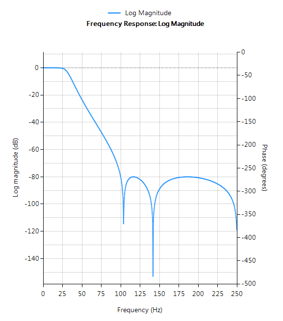
Elliptic
Elliptic filters offer steeper roll-off characteristics than Butterworth or Chebyshev filters, but are equiripple in both the passband and the stopband. In general, Elliptic filters meet the design specifications with the lowest order of any of the methods discussed herein.
Filter characteristics
- Fastest roll-off of all supported prototypes
- Equiripple in both the passband and stopband
- Lowest order filter of all supported prototypes
- Non-linear passband phase characteristics
- Good choice for real-time control and high-throughput (RF applications) applications
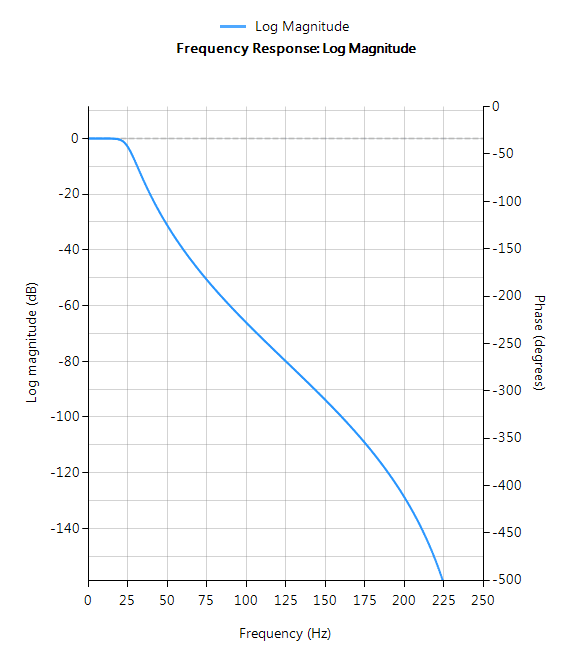
Butterworth
Butterworth filters have a magnitude response that is maximally flat in the passband and monotonic overall, making them a good choice for DC and low frequency measurement applications, such as loadcells. However, this highly desirable ‘smoothness’ comes at the price of decreased roll-off steepness. As a consequence, the Butterworth method has the slowest roll-off characteristics of all the methods discussed herein.
Filter characteristics
- Smooth monotonic response (no ripple)
- Slowest roll-off for equivalent order
- Highest order of all supported prototypes
- More linear passband phase response than all other methods
- Good choice for DC measurement and audio applications
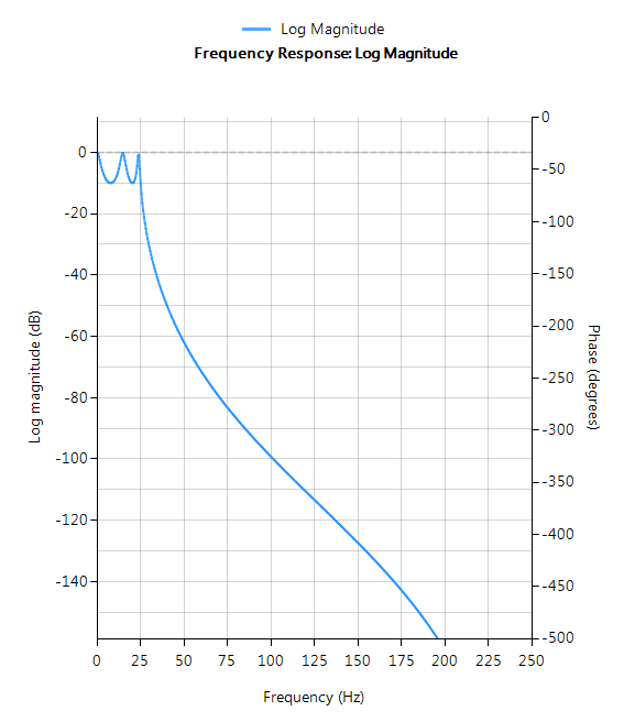
Chebyshev Type I
Chebyshev Type I filters are equiripple in the passband and monotonic in the stopband. As such, Type I filters roll off faster than Chebyshev Type II and Butterworth filters, but at the expense of greater passband ripple.
Filter characteristics
- Passband ripple
- Maximally flat stopband
- Faster roll-off than Butterworth and Chebyshev Type II
- Good compromise between Elliptic and Butterworth
Chebyshev Type II
Chebyshev Type II filters are monotonic in the passband and equiripple in the stopband making them a good choice for bridge sensor applications. Although filters designed using the Type II method are slower to roll-off than those designed with the Chebyshev Type I method, the roll-off is faster than those designed with the Butterworth method.
Filter characteristics
- Maximally flat passband
- Faster roll-off than Butterworth
- Slower roll-off than Chebyshev Type I
- Good choice for DC measurement applications