Did you know that there are 23 billion IoT embedded devices currently deployed around the world? This figure is expected to grow to a whopping 1 trillion devices by 2050!

Less known, is that 80% of IoT devices are based around Arm’s Cortex-M microcontroller technology. Sometimes clients ask us if we support their Arm Cortex-M based demo-board of choice. The answer is simply: yes!

200+ IC vendors supported

The ASN Filter Designer has an automatic code generator for Arm Cortex-M cores, which means that we support virtually every Arm based demo-board: ST, Cypress, NXP, Analog Devices, TI, Microchip/Atmel and over 200+ other manufacturers. Our compatibility with Arm’s free CMSIS-DSP software framework removes the frustration of implementing complicated digital filters in your IoT application – leaving you with code that is optimal for Cortex-M devices and that works 100% of the time.

The Arm Cortex-M family of microcontrollers are an excellent match for IoT applications. Some of the advantages include:

  • Low power and cost – essential for IoT devices
  • Microcontroller with DSP functionality all-in-one
  • Embedded hardware security functionality
  • Cortex-M4 and M7 cores with hardware floating support (enhanced microcontrollers)
  • Freely available CMSIS-DSP C library: supporting over 60 signal processing functions

Automatic code generation for Arm’s CMSIS-DSP software framework

Simply load your sensor data into the ASN Filter Designer signal analyser and perform a detailed analysis. After identifying the wanted and unwanted components of your signal, design a filter and test the performance in real-time on your test data. Export the designed design to Arm MDK, C/C++ or integrate the filter into your algorithm in another domain, such as in Matlab, Python, Scilab or Labview.

Use the tool in your RAD (rapid application development) process, by taking advantage of the automatic code generation to Arm’s CMSIS-DSP software framework, and quickly integrate the DSP filter code into your main application code.

Let the tool analyse your design, and automatically generate fully compliant code for either the M0, M0+, M3, M4 and the newer M23 and M33 Cortex cores. Deploy your design within minutes rather than hours.

Proud Arm knowledge partner

We are proud that we are an Arm knowledge partner! As an Arm DSP knowledge partner, we will be kept informed of their product roadmap and progress for the coming years.

Try it for yourself and see the benefits that the ASN Filter Designer can offer your organisation by cutting your development costs by up to 75%!

How to choose between analog signal processing (ASP) and digital signal processing (DSP). How too chose for ASP or DSP; analog filters or digital filters?


Drones and DC motor control – How the ASN Filter Designer can save you a lot of time and effort

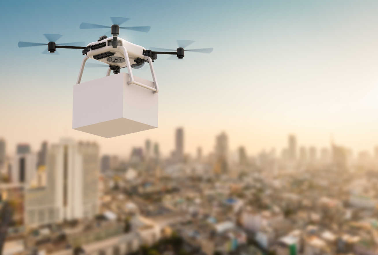
Drones are one of the golden nuggets in IoT. No wonder, they can play a pivotal role in congested cities and far away areas for delivery. Further, they can be a great help to give an overview of a large area or places which are difficult or dangerous to reach. However, most of the technology is still in its experimental stage.

Because drones have a lot of sensors, Advanced Solutions Nederland did some research on how drone producing companies have solved questions regarding their sensor technology, especially regarding DC motor control.

Until now: solutions developed with great difficulty

We found out that most producers spend weeks or even months on finding solutions for their sensor technology challenges. With the ASN Filter Designer, he/she could have come to a solution within days or maybe even hours. Besides, we expect that the measurement would be better too.

The biggest time coster is that until now algorithms were developed by handwork, i.e. they were developed in a lab environment and then tested in real-life. With the result of the test, the algorithm would be tweaked again until the desired results were reached. However, yet another challenge stems from the fact that a lab environment is where testing conditions are stable, so it’s very hard to make models work in real life. These steps result in rounds and rounds of ‘lab development’ and ‘real life testing’ in order to make any progress -which isn’t ideal!

How the ASN Filter Designer can help save a lot of time and effort

The ASN Filter Designer can help a lot of time in the design and testing of algorithms in the following ways:

  • Design, analyse and implement filters for drone sensor applications with real-time feedback and our powerful signal analyser.
  • Design filters for speed and positioning control for sensorless BLDC (brushless DC) motor applications.
  • Speed up deployment to Arm Cortex-M embedded processors.


Real-time feedback and powerful signal analyser

One of the key benefits of the ASN Filter Designer and signal analyser is that it gives real-time feedback. Once an algorithm is developed, it can easily be tested on real-life data. To analyse the real-life data, the ASN Filter Designer has a powerful signal analyser in place.

Design and analyse filters the easy way

You can easily design, analyse and implement filters for a variety of drone sensor applications, including: loadcells, strain gauges, torque, pressure, temperature, vibration, and ultrasonic sensors and assess their dynamic performance in real-time for a variety of input conditions.  With the ASN Filter Designer, you don’t have do to any coding yourself or break your head with specifications: you just have to draw the filter magnitude specification and the tool will calculate the coefficients itself.

Speed up deployment

Perform detailed time/frequency analysis on captured test datasets and fine-tune your design. Our Arm CMSIS-DSP and C/C++ code generators and software frameworks speed up deployment to a DSP, FPGA or micro-controller.

An example: designing BLDC motor control algorithms

BLDC (brushless DC) BLDC motors have found use in a variety of application areas, including: robotics, drones and cars. They have significant advantages over brushed DC motors and induction motors, such as: better speed-torque characteristics, high reliability, longer operating life, noiseless operation, and reduction of electromagnetic interference (EMI).

One advantage of BLDC motor control compared to standard DC motors is that the motor’s speed can be controlled very accurately using six-step commutation, making it a good choice for precision motion applications, such as robotics and drones.

Sensorless back-EMF and digital filtering

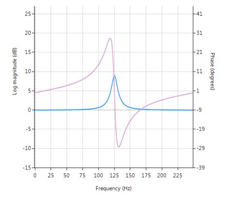
For most applications, monitoring of the back-EMF (back-electromotive force) signal of the unexcited phase winding is easier said than done, since it has significant noise distortion from PWM (pulse width modulation) commutation from the other energised windings. The  coupling  between  the  motor parameters, especially inductances, can induce ripple in the back-EMF signal that is synchronous with the PWM commutation.  As a consequence, this induced ripple on the back EMF signal leads to faulty commutation. Thus, the measurement challenge is how to accurately measure the zero-crossings of the back-EMF signal in the presence of PWM signals?

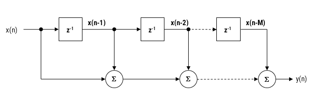
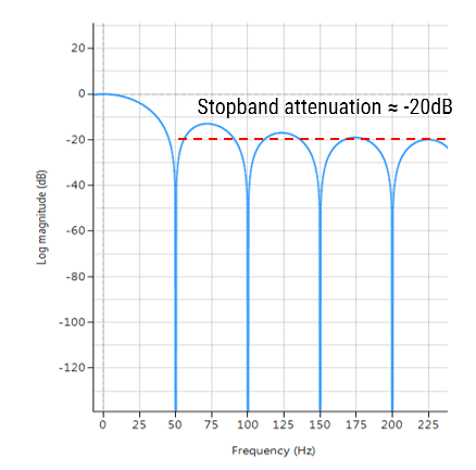
A standard solution is to use digital filtering, i.e. IIR, FIR or even a median (majority) filter. However, the challenge for most designers is how to find the best filter type and optimal filter specification for the motor under consideration.

The solution

The ASN Filter Designer allows engineers to work on speed and position sensorless BLDC motor control applications based on back-EMF filtering to easily experiment and see the filtering results on captured test datasets in real-time for various IIR, FIR and median (majority filtering) digital filtering schemes. The tool’s signal analyser implements a robust zero-crossings detector, allowing engineers to evaluate and fine-tune a complete sensorless BLDC control algorithm quickly and simply.

So, if you have a measurement problem, ask yourself:

Can I save time and money, and reduce the headache of design and implementation with an investment in new tooling?

Our licensing solutions start from just 125 EUR for a 3-month licence.

Find out what we can do for you, and learn more by visiting the ASN Filter Designer’s product homepage.

All-pass filters

All-pass filters provide a simple way of altering/improving the phase response of an IIR without affecting its magnitude response. As such, they are commonly referred to as phase equalisers and have found particular use in digital audio applications.

In its simplest form, a filter can be constructed from a first order transfer function, i.e.,

\( A(z)=\Large{\frac{r+z^{-1}}{1+r z^{-1}}}  \, \,  \normalsize{; r<1} \)

Analysing \(\small A(z)\), notice that the pole and zero lie on the real z-plane axis and that the pole at radius \(\small r\) has a zero at radius \(\small 1/r\), such that the poles and zeros are reciprocals of another. This property is key to the all-pass filter concept, as we will now see by expanding the concept further to a second order all-pass filter:

\( A(z)=\Large\frac{r^2-2rcos \left( \frac{2\pi f_c}{fs}\right) z^{-1}+z^{-2}}{1-2rcos \left( \frac{2\pi f_c}{fs}\right)z^{-1}+r^2 z^{-2}} \)

Where, \(\small f_c\) is the centre frequency, \(\small r\) is radius of the poles andall pass filter, all-pass filter, allpass filter, all pass pole-zero \(\small f_s\) is the sampling frequency. Notice how the numerator and denominator coefficients are arranged as a mirror image pair of one another.  The mirror image property is what gives the all-pass filter its desirable property, namely allowing the designer to alter the phase response while keeping the magnitude response constant or flat over the complete frequency spectrum.

all pass filter, all-pass filter, allpass, phase equaliser, altering/improving the phase response of an IIR without affecting its magnitude responseFrequency response of all-pass filter:
Notice the constant magnitude spectrum (shown in blue).

Implementation

An All-pass filter may be implemented in ASN FilterScript as follows:

ClearH1;  // clear primary filter from cascade

interface radius = {0,2,0.01,0.5};   // radius value
interface fc = {0,fs/2,1,fs/10};     // frequency value

Main()
Num = {radius^2,-2*radius*cos(Twopi*fc/fs),1};
Den = reverse(Num); // mirror image of Num
Gain = 1;

For a detailed discussion on IIR filter phase equalisation, and the ASN Filter designer’s APF (all-pass filter) design tool, please refer to the following article.

ASN Filter Designer DSP


Download demo now

Licencing information

Author

  • Dr. Sanjeev Sarpal

    Sanjeev is an AIoT visionary and expert in signals and systems with a track record of successfully developing over 25 commercial products. He is an Arm Ambassador and advises top international blue chip companies on their AIoT solutions and strategies for I4.0, telemedicine, smart healthcare, smart grids and smart buildings.

A  Peaking or Bell filter is a type of audio equalisation filter that boosts or attenuates the magnitude of a specified set of frequencies around a centre frequency in order to perform magnitude equalisation. As seen in the plot in the below, the filter gets its name from the shape of the its magnitude spectrum (blue line) which resembles a Bell curve.

Peaking filter or Bell filter, a type of audio equalisation filter that boosts or attenuates the magnitude of a specified set of frequencies around a centre frequency in order to perform magnitude equalisation. As seen in the plot in the below, the filter gets its name from the shape of the its magnitude spectrum (blue line) which resembles a Bell curve.

Frequency response (magnitude shown in blue, phase shown in purple) of a 2nd order Bell filter peaking at 125Hz.

All-pass filters

Central to the Bell filter is the so called All-pass filter. All-pass filters provide a simple way of altering/improving the phase response of an IIR without affecting its magnitude response. As such, they are commonly referred to as phase equalisers and have found particular use in digital audio applications.

A second order all-pass filter is defined as:

\( A(z)=\Large\frac{r^2-2rcos \left( \frac{2\pi f_c}{fs}\right) z^{-1}+z^{-2}}{1-2rcos \left( \frac{2\pi f_c}{fs}\right)z^{-1}+r^2 z^{-2}} \)

Notice how the numerator and denominator coefficients are arranged as a mirror image pair of one another.  The mirror image property is what gives the all-pass filter its desirable property, namely allowing the designer to alter the phase response while keeping the magnitude response constant or flat over the complete frequency spectrum.

A Bell filter can be constructed from the \(A(z)\) filter by the following transfer function:

\(H(z)=\Large\frac{(1+K)+A(z)(1-K)}{2}\)

After some algebraic simplication, we obtain the transfer function for the Peaking or Bell filter as:

\(H(z)=\Large{\frac{1}{2}}\left[\normalsize{(1+K)} + \underbrace{\Large\frac{k_2 + k_1(1+k_2)z^{-1}+z^{-2}}{1+k_1(1+k_2)z^{-1}+k_2 z^{-2}}}_{all-pass filter}\normalsize{(1-K)} \right] \)

  • \(K\) is used to set the gain and sign of the peak
  • \(k_1\) sets the peak centre frequency
  • \(k_2\) sets the bandwidth of the peak

Implementation

A Bell filter may easily be implemented in ASN FilterScript as follows:

ClearH1;  // clear primary filter from cascade
interface BW = {0,2,0.1,0.5}; // filter bandwidth
interface fc = {0, fs/2,fs/100,fs/4}; // peak/notch centre frequency
interface K = {0,3,0.1,0.5}; // gain/sign

Main()

k1=-cos(2*pi*fc/fs);
k2=(1-tan(BW/2))/(1+tan(BW/2));

Pz = {1,k1*(1+k2),k2}; // define denominator coefficients
Qz = {k2,k1*(1+k2),1}; // define numerator coefficients
Num = (Pz*(1+K) + Qz*(1-K))/2;
Den = Pz;
Gain = 1;

This code may now be used to design a suitable Bell filter, where the exact values of \(K, f_c\) and \(BW\) may be easily found by tweaking the interface variables and seeing the results in real-time, as described below.

Designing the filter on the fly

Central to the interactivity of the FilterScript IDE (integrated development environment) are the so called interface variables. An interface variable is simply stated: a scalar input variable that can be used modify a symbolic expression without having to re-compile the code – allowing designers to design on the fly and quickly reach an optimal solution.

As seen in the code example above, interface variables must be defined in the initialisation section of the code, and may contain constants (such as, fs and pi) and simple mathematical operators, such as multiply * and / divide. Where, adding functions to an interface variable is not supported.

An interface variable is defined as vector expression:

interface name = {minimum, maximum, step_size, default_value};

Where, all entries must be real scalars values. Vectors and complex values will not compile.

Real-time updates

All interface variables are modified via the interface variable controller GUI. After compiling the code, use the interface variable controller to tweak the interface variables values and see the effects on the transfer function. If testing on live audio, you may stream a loaded audio file and adjust the interface variables in real-time in order to hear the effects of the new settings.

Comb filters: powerline (50/60Hz) harmonic cancellation filters, audio applications; cascaded integrator–comb (CIC) filters: anti-aliasing, anti-imaging

FIR Farrow delay filter: nudge or fine-tune the sampling instants by a fraction of a sample. May be May be combined with traditional integer delay line

The moving average (MA) filter is perhaps one of the most widely used FIR filters due to its conceptual simplicity and ease of implementation. As seen in the diagram below, notice that the filter doesn’t require any multiplications, just additions and a delay line, making it very suitable for many extreme low-power embedded devices with basic computational capabilities.

fir direct form

However, despite its simplicity, the moving average filter is optimal for reducing random noise while retaining a sharp step response, making it a versatile building block for smart sensor signal processing applications.

A moving average filter of length \(L\) for an input signal \(x(n)\) may be defined as follows:

\(y(n)=\large{\frac{1}{L}}\normalsize{\sum\limits_{k=0}^{L-1}x(n-k)}\) for \(\normalsize{n=0,1,2,3….}\)

Where, a simple rule of thumb states that the amount of noise reduction is equal to the square-root of the number of points in the average. For example, an MA of length 9 will result in a factor 3 noise reduction.

moving average filterFrequency response of an MA filter of length 9. Notice the poor stopband attentuation at around -20dB.

Advantages

  • Most commonly used digital lowpass filter.
  • Optimal for reducing random noise while retaining a sharp step response.
  • Good smoother (time domain).
  • Unity valued filter coefficients, no MAC (multiply and accumulate) operations required.
  • Conceptually simple to implement.

Disadvantages

  • Inflexible frequency response: nudging a conjugate zero pair results in non-unity coefficients.
  • Poor lowpass filter (frequency domain): slow roll-off and terrible stopband attenuation characteristics.

Implementation

The MA filter may be implemented in ASN FilterScript as follows:

ClearH1;  // clear primary filter from cascade
Main();
Hd=movaver(8,"symbolic");  // design an 8th order MA
Num = getnum(Hd);   // define numerator coefficients
Den = {1};          // define denominator coefficients
Gain = getgain(Hd); // define gain

A more computationally efficient implementation of the MA filter is discussed here.

Further reading

  • Understanding Digital Signal Processing, Chapter 5, R. G. Lyons
  • The Scientist and Engineer’s Guide to Digital Signal Processing, Chapter 15, Steven W. Smith

Download demo now

Licencing information