AIoT is an exciting new area that combines AI concepts (i.e. ML) with IoT in order to produce state-of-the-art smart embedded solutions. This augmentation of technologies requires a new set of tools to capture real-time IoT sensor data, analyse it, design suitable algorithms and then perform validation of the solution.  After completing validation of the algorithms on the test data, a final hurdle is then how to generate efficient C code of the developed algorithm(s) for an Arm Cortex-M microcontroller for use in an application. These concepts will be discussed herein.

Arm’s Synchronous Data Stream (SDS) Framework provides developers with an easy method of capturing and playing back real-time sensor data for embedded AIoT sensor applications on Arm Cortex-M processors, such as ST Microelectronics’ very popular STM32 family.

The SDS Framework provides embedded developers with a variety of essential tools, such as the ability to record real-world sensor data for analysis and development in tools such as ASN Filter Designer, Python and Matlab. A set of Python utility scripts are available for recording, playback, visualisation and data conversion, where the latter supports the conversion of captured SDS data files into a single CSV file – providing a simple bridge between the ASN Filter Designer and the SDS Framework.

The SDS framework also supports the possibility to playback real-world data for algorithm validation using Arm Virtual Hardware, allowing developers to verify execution of DSP algorithms on Cortex-M targets with off-line tools.

This application note provides AIoT developers with a complete reference guide of how to develop and deploy feature extraction algorithms for use in AIoT applications to STM32 Arm Cortex-M based microcontrollers using STM32CubeIDE or Keil mVision with the Arm SDS framework and ASN Filter Designer. As mentioned above, AIoT system challenges and concepts will also be covered.

Building AIoT systems

Almost all IoT embedded sensor applications require some level of signal processing to enhance sensor data and extract features of interest. However, an obvious hurdle for many developers is how to design, test and deploy efficient algorithms for their application. This is easier said than done, as many software engineers are not well-versed in understanding the mathematical concepts needed to implement algorithms. This is further complicated by the challenge of how to implement algorithms developed by researchers that are not interested/experienced in developing real-time embedded applications.

A possible solution offered by the Mathworks (Embedded Coder) automatically translates Matlab algorithms and functions into C for Arm processors, but its high price tag and steep learning curve make it unattractive for many.

That being said, Arm and its rich ecosystem of partners provide developers with extensive easy-to-use tooling and tried and tested software libraries. Arm’s CMSIS-DSP and CMSIS-NN frameworks for algorithm development and machine learning (ML) are two very popular examples that are open source and are used internationally by tens of thousands of developers.

The Arm CMSIS-DSP software framework is particularly interesting as it provides IoT developers with a rich collection of fast mathematical and vector functions, interpolation functions, digital filtering (FIR/IIR) and adaptive filtering (LMS) functions, motor control functions (e.g. PID controller), complex math functions and supports various data types, including fixed and floating point. The important point to make here is that all of these functions have been optimised for Arm Cortex-M processors, allowing you to focus on your application rather than worrying about optimisation.  

The Arm-CMSIS framework solutions are strengthened by Arm partners ASN and Qeexo who provide developers with easy-to-use real-time filtering, feature extraction (ASN Filter Designer) and ML tooling (AutoML) and reference designs, expediting the development of AIoT applications, including industrial, audio and biomedical. These solutions have been optimised for Arm processors with the help of Arm’s architecture experts and insider knowledge of compiler workings.

AIoT system building blocks

An essential pre-building block in any AIoT system is the feature extraction algorithm. The challenge for any feature extraction algorithm is to extract and enhance any relevant sensor data features in noisy or undesirable circumstances and then pass them onto the ML model in order to provide an accurate classification.  The concept is illustrated below:

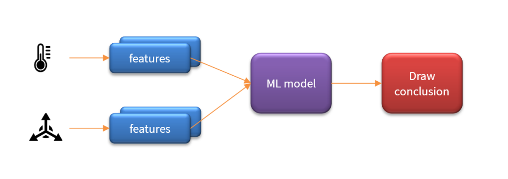
As seen above, an AIoT system may actually contain multiple feature blocks per sensor and in some cases fuse the features locally before sending them onto the ML model for classification such that the system may then draw a conclusion. The challenge is therefore how to capture sensor data for training and design suitable algorithms to extract features of interest.

Feature extraction algorithms: challenges and solutions

The challenge for any feature extraction algorithm is to extract and enhance any relevant data features in noisy data or undesirable circumstances and then pass them onto the ML model in order to provide an accurate classification. Unfortunately, many ML models perform badly, due to poor quality data and insufficient training data.   An obvious challenge for AIoT is how do we obtain the training data in the first place? In many cases, this is extremely challenging as data pertaining to faults (such as preventive maintenance) is hard to come by, as many plant managers are reluctant to break their working production lines or processes to provide developers with training data.

In the absence of adequate training data, feature extraction based on science and mathematics is a prudent alternative, as less training data is required, and in general, the quality of the feature estimate is higher as knowledge of the underlying process is used. Examples include: obtaining accurate pulse and heart rate estimates from ECG and PPG sensors in smartwatch applications when a subject is moving.  For industrial sensors, such as loadcells, pressure, temperature, gas and accelerometer sensors the challenge is amplified, as harsh operating conditions and the sheer variety of the applications needed for I4.0 process control applications complicate the design significantly.

Example: Infrared gas sensor

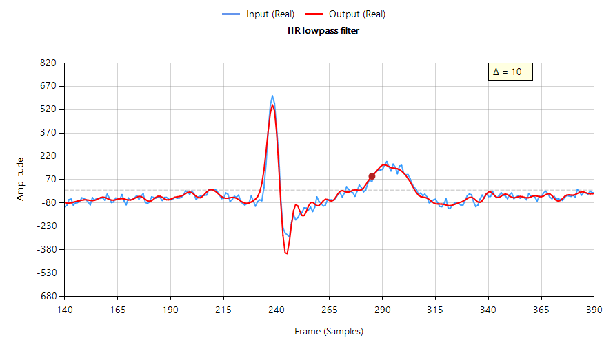
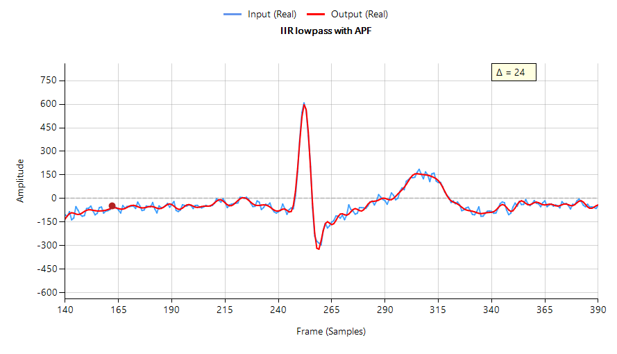
Consider the following application for gas concentration measurement from an Infrared gas sensor. The requirement is to determine the peak-to-peak amplitude of the sinusoid in order to get an estimate of gas concentration – where the bigger amplitude is the higher the gas concentration will be.

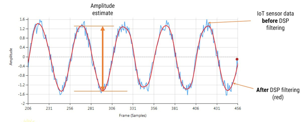
Analysing the Figure, it can be seen that the sinusoid is corrupted with measurement noise (shown in blue), and any estimate based on the blue signal will have a high degree of uncertainty about it – which is not very useful for getting an accurate reading of gas concentration! After cleaning the sinusoid with a digital filter (red line), we obtain a much more accurate and usable signal for our gas concentration estimation challenge. But how do we obtain the amplitude?

Knowing that the gradient at the peaks is zero, a relatively easy and robust way of finding the peaks of the sinusoid is via numerical differentiation, i.e. computing the difference between sample values and then looking for the zero-crossing points in the differentiated data. Armed with the positions and amplitudes of the peaks, we can take the average and easily obtain the amplitude and frequency.  Notice that any DC offsets and low-frequency baseline wander will be removed via the differentiation operation.

This is just a simple example of how to extract the properties of a sinusoid in real-time using science and mathematics and an understanding of the underlying process without the need for ML training data.

AIoT feature extraction smart sensor design workflow

Arm’s Synchronous Data Stream (SDS) Framework provides developers with an easy method of capturing and playing back real-time sensor data for embedded AIoT sensor applications on Arm Cortex-M processors. A set of Python utility scripts are available for recording, playback, visualisation and data conversion, where the latter supports the conversion of captured SDS data files into a single CSV file – providing a simple bridge between the ASN Filter Designer and the SDS Framework.

An AIoT smart sensor design workflow using the ASN Filter Designer and the SDS Framework is shown below.

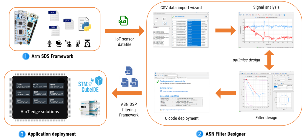
As seen above, three major components constitute the AIoT design workflow.

  1. Arm SDS Framework: capturing IoT sensor data and converting it to CSV format.
  2. ASN Filter Designer: importing the CSV datafile and then analysing the data. Based on the data analysis, a suitable filter can be designed together with other filters and IP blocks in order to build feature extraction algorithms for ML applications.
  3. Application deployment: Generating optimised C code and combining the design with an application for use on an Arm microcontroller.

The SDS Framework can be used with all major demo boards, including ST’s Discovery kit and Nucleo boards. SDS Python utilities are used to convert the captured *.sds and *.yaml files into a CSV file for import into the ASN Filter Designer, as discussed in the following section.

Data Import Wizard

The ASN Filter Designer’s comprehensive data import wizard can delimitate and import a variety of multi-column IoT datasets in CSV or TXT form.

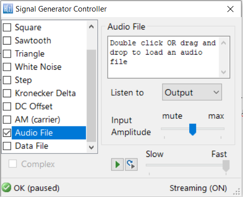
As seen in the video, a generated CSV file can be dragged and dropped onto the signal analyser canvas, bringing up the data import wizard. The import wizard will automatically check the imported data for errors (such as NaNs, Infs etc) and then order the data into columns. Any header line data can be skipped by setting the Skip Headerlines value respectively.

For the example considered herein, the data is actually triaxial accelerometer data (i.e. X, Y and Z axes) with an extra column for the timebase. Therefore, if we wish to import the X-axis data, we can simply click on the header for the second column (B).   The tool will then ask you to recheck the data, and upon clicking on ‘Save’ will save the selected data as a single-column CSV file (needed for the ASN Filter Designer). This new CSV file can then be streamed via the tool’s signal generator for algorithm development.

Deploying to Arm Cortex-M processors

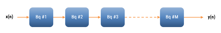
After completing the design process, the designed filter(s) can be deployed to STM32CubeIDE or Arm/Keil uVision for integration into an application project. Depending on the functionality of the ASN Filter Designer’s signal chain, two software frameworks are available: Arm’s CMSIS-DSP and ASN’s ANSI C DSP.

The ANSI C DSP framework was developed with close collaboration with Arm’s architecture team, providing outstanding computational performance that is required for real or complex coefficient floating-point designs that use multiple filters and mathematical functions in a signal chain. The Arm CMSIS-DSP framework on the other hand is an excellent choice for implementing both fixed-point and floating-point filters, but is limited to real coefficient single FIR filter or one IIR Biquad cascade with no extra mathematical functions.

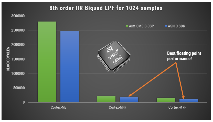
A benchmark comparison for both frameworks is shown below for an 8th IIR filter running on three different Arm cores. As seen, the ASN Framework is slightly faster (lower means better performance) than the Arm Framework.

Framework Benchmarks: lower number of clock cycles means higher performance.

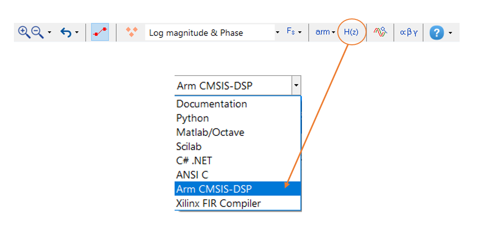
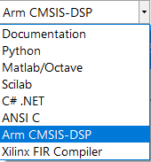
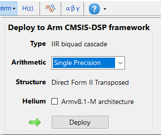
Arm CMSIS-DSP wizard

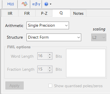
Professional licence users may expedite the deployment by using the Arm deployment wizard. The tool will automatically analyse your design and choose a suitable Framework. If the design cannot be exported via the Arm CMSIS-DSP framework, the tool will suggest that you use the ASN ANSI C framework and launch the code generation wizard.

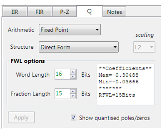
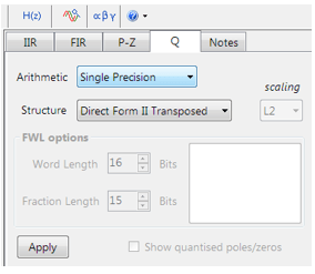
Note that the built-in AI will automatically determine the best settings for your design based on the quantisation settings chosen.

Clicking on Deploy will automatically analyse your complete filter cascade and convert any extra filters in the cascade into an H1 (primary) for implementation. Upon completion, the tool will then launch the C code generation wizard.

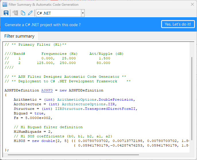
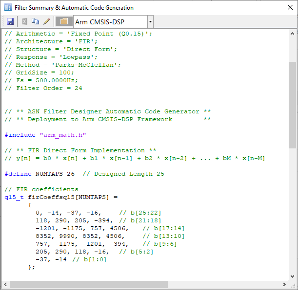
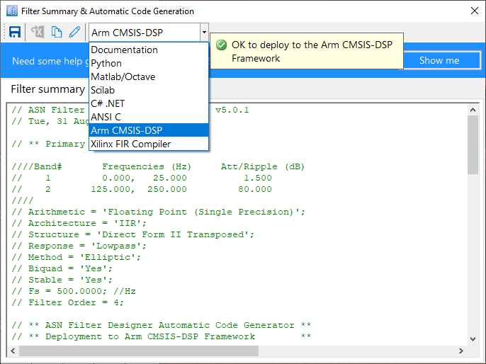
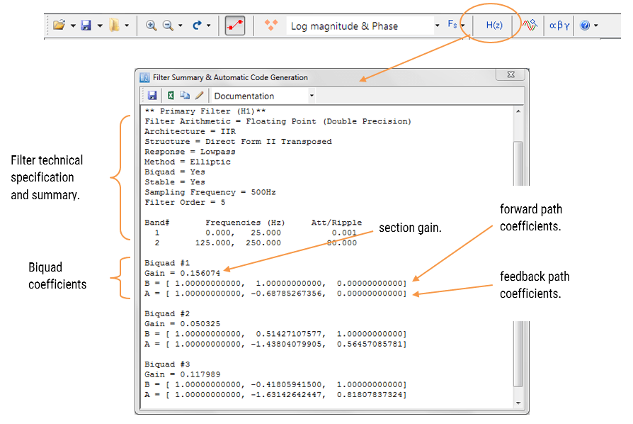
CMSIS-DSP C code generation

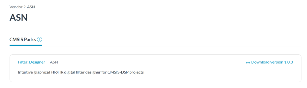
Depending on which C framework is used, the C code generator wizard will automatically generate the C code needed for your design. For developers using the Arm CMSIS-DSP framework, a single C file is generated for use with an MDK5 software pack. The MDK5 pack is available from Arm Keil’s software pack repository, providing several complete filtering examples based on the ASN Filter Designer’s code generator using the Arm CMSIS-DSP library.

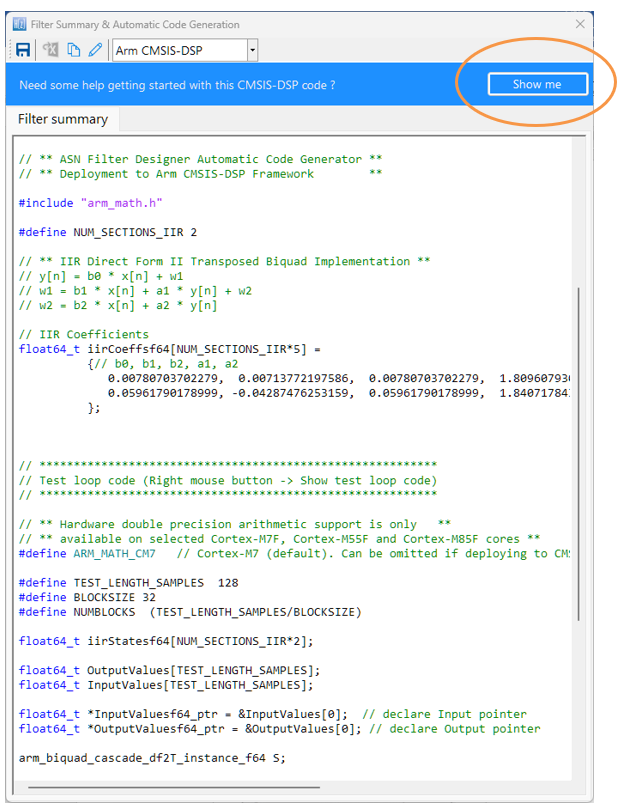
A detailed help tutorial is available by clicking on the Show me button. 

ASN ANSI C DSP code generation

For developers using the ASN ANSI C DSP framework, the code wizard should be used.

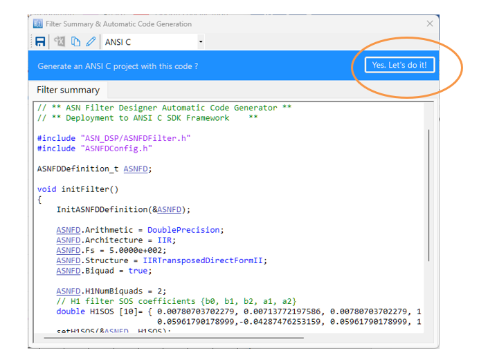
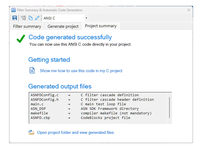
NB. The wizard will produce a CodeBlocks project in order to get you started. The following section describes in detail the steps needed for using the generated code in a STM32CUBE-IDE project. Please refer to the ANSI C SDK user guide for step-by-step instructions on how to use the generated code in other IDEs. 

A PDF version of this article is available as an application note.

Author

  • Dr. Sanjeev Sarpal

    Sanjeev is an AIoT visionary and expert in signals and systems with a track record of successfully developing over 25 commercial products. He is a Distinguished Arm Ambassador and advises top international blue chip companies on their AIoT solutions and strategies for I4.0, telemedicine, smart healthcare, smart grids and smart buildings.

Over the decades Microsoft has produced various programming languages (e.g. C#, F#, Visual Basic) and flavours of their .NET paradigm, such as the very popular 4.x .NET Framework.  

C# is very popular among Windows developers, as it is based on objected orientated programming concepts together with a few other pearls, such as automatic memory management (something that had to be handled manually in C++), in an attempt to provide many of the advantages of C++ in a much more simplified way.

These pros combined with the .NET Framework’s extensive charting library, UI toolbox, Networking, ML engine libraries and general ease of use in Microsoft Visual Studio was one of the primary reasons that many Windows-based scientific programs (e.g. ASN Filter Designer) were developed using the C# language and .NET Framework.

Over the last few years, Microsoft has tried to consolidate their .NET solution into a single, fast, cross-platform solution with the advent of the .NET Core paradigm. .NET Core is an open-source framework for developing Windows, web applications, services, and mobile applications and it can be run on Windows, Mac and Linux. Microsoft contends that .NET Core is much faster than the .NET Framework since the architecture has been completely rewritten to make it modular, lightweight, fast and cross-platform compatible.

DSP filtering library for C# .NET applications

For many modern scientific applications digital filtering of datasets is just one of the many components needed for an algorithm. This could be extracting ECG and PPG biomedical features, cancelling powerline interference or removing the noise from a dataset. In many cases, it is desirable to perform the filtering in real-time on streaming data as part of an algorithm updating dashboard analytics.

ASN Filter Designer provides .NET developers with an automatic code generator and SDK for developing high-performance data filtering applications in C#.

The tool’s project wizard bundles all of the necessary SDK framework files needed to run a designed filter cascade without the need for any other dependencies or 3rd party plugins. The deployed code is fully compatible with Microsoft Visual Studio and all .NET versions.

A complete overview of the SDK is available here.


Download demo now

Licencing information

Author

  • Dr. Sanjeev Sarpal

    Sanjeev is an AIoT visionary and expert in signals and systems with a track record of successfully developing over 25 commercial products. He is a Distinguished Arm Ambassador and advises top international blue chip companies on their AIoT solutions and strategies for I4.0, telemedicine, smart healthcare, smart grids and smart buildings.

ASN Filter Designer’s ANSI C SDK framework, provides developers with a comprehensive C code framework for developing  AIoT filtering application on microcontrollers and embedded platforms. Although the framework has been primarily designed to support the just ASN filter Designer’s filter cascade, it is possible to create extra filter objects to augment the cascade.

Two common filtering methods used by AIoT developers are the Median and moving average (MA) filters. Although these fully integrated within the Framework’s filter cascade, it is often useful to have the flexibility of an additional filtering block to act as a post filter smoothing filter.

An extra median or MA filter may be easily added to main.c as shown below. Notice that data is filtered in blocks of 4 as required by the framework.

Median filter

The Median filter is non-linear filtering method that uses the concept of majority voting (i.e. calculating the median) to remove glitches and smooth data.  It is edge preserving, making it a good choice for enhancing square waves or pulse like data.

 
#include "ASN_DSP/DSPFilters/MedianFilter.h"
float InputTemp[4];
float OutputTemp[4];

MedianFilter_t MyMedianfilter;

InitMedianFilter(&MyMedianfilter,7);  // median of length 7

   for (n=0; n<TEST_LENGTH_SAMPLES; n+=4)
   {
        InputTemp[0]=InputValues[n];
        InputTemp[1]=InputValues[n+1];
        InputTemp[2]=InputValues[n+2];
        InputTemp[3]=InputValues[n+3];

        MedianFilterData(&MyMedianfilter,InputTemp, OutputTemp);

        OutputValues[n]=OutputTemp[0];
        OutputValues[n+1]=OutputTemp[1];
        OutputValues[n+2]=OutputTemp[2];
        OutputValues[n+3]=OutputTemp[3];
   }

Moving Average filter

The moving average (MA) filter is optimal for reducing random noise while retaining a sharp step response, making it a versatile building block for smart sensor signal processing applications. It is perhaps one of the most widely used digital filters due to its conceptual simplicity and ease of implementation.

 
#include "ASN_DSP/DSPFilters/MAFilter.h"
float InputTemp[4];
float OutputTemp[4];

MAFilter_t MyMAfilter;

InitMAFilter(&MyMAfilter,9);  // MA of length 9

   for (n=0; n<TEST_LENGTH_SAMPLES; n+=4)
   {
       InputTemp[0]=InputValues[n];
       InputTemp[1]=InputValues[n+1];
       InputTemp[2]=InputValues[n+2];
       InputTemp[3]=InputValues[n+3];

       MAFilterData(&MyMAfilter,InputTemp, OutputTemp);

       OutputValues[n]=OutputTemp[0];
       OutputValues[n+1]=OutputTemp[1];
       OutputValues[n+2]=OutputTemp[2];
       OutputValues[n+3]=OutputTemp[3];
   }

Download demo now

Licencing information


Author

  • Marty de Vries

    Marty is an applications engineer and embedded software expert at ASN. He has over 10 years experience in developing high performance embedded libraries and applications for Arm processors.

An all-pass equalisation filter cascade (Heq) is available for equalising the phase response of the H1 filter cascade and H2 filter respectively.

Many Audio/acoustics engineers, researchers and audio hobbyists work with DSP (Digital Signal Processing). In this article, you’ll find out how the ASN Filter Designer helps both experienced audio engineers and engineers where DSP is not their daily job to create digital filters for audio and speech.

For whom?

If you are an audio/acoustics engineer, researcher or even a hobbyist with a little bit of DSP knowledge: ASN Filter Designer is for you! The tool offers the following benefits:

  • Intuitive and easy to use.
  • Logarithmic frequency axis.
  • Save days of time spending calculating on your own for the price of 2-3 hours of work.
  • Few lesser costs then extensive tooling with features you don’t use anyway.
  • Automatic code generation: export for further analysis to Matlab, etc, or to Cortex-M Arm based processors via the Arm CMSIS-DSP software framework.

How DSP for Speech and audio benefit from ASN Filter Designer:

  • Experiment with a variety of equalisation, noise cancellation and sound effect audio filtering algorithms.
  • Perform data analysis in the frequency domain and via specialised methods, including Cepstral analysis on the streaming data.
  • Import your own wav audio files (mono or stereo up to 48kHz) for streaming, and modify the filter characteristics in real-time while listening to the filtered audio stream.

Some features for creating digital filters for Audio and Speech:


Sampling frequency

The sampling frequency may be specified up to 4 decimal places

This is useful for designing filters based on fractional sampling frequencies, such as multiples of the 44.1kHz audio standard. Common examples include audio interpolation filters: 44.1kHz × 128 = 5.6448MHz and 44.1kHz × 256 = 11.2896MHz.

Filter orders of up to 499

Long FIR filters may be constructed, where this is limited to 200 for streaming audio applications.

Logarithmic frequency axis

Perform detailed analysis across the complete audio spectrum 20Hz-20kHz.   

Audio and user data playback streaming

Signal Generator Controller: 
Choose what you want to listen to; Adjust the amplitude of the input signal
Signal Generator Controller:
Choose what you want to listen to; Adjust the amplitude of the input signal

The signal analyzer allows designers to test their design on audio, real (user) data or synthetic data via the built-in signal generator. Default data playback is implemented as streaming data, providing a simple way of assessing the filter’s dynamic performance, which is especially useful for fixed point implementations. Both frequency domain and time domain charts are fully supported, allowing for design verification via transfer function estimation using the cross and power spectral density functions. As with all other charts, the signal analyzer chart fully supports advanced zooming and panning, as well as comprehensive chart data file export options.

Load .wav for playback

The signal generator allows you to load .wav audio files for playback via the Audio File method. Both mono and stereo formats are fully supported for 8.000, 11.025, 16.000, 22.05, 44.1 and 48kHz. sampling rates. There is no restriction as to the length of the .wav file.

You may add extra signals to input audio stream

Use the signal generator to add sinewaves and white noise to the data stream.

Intuitive data analysis with the mouse

Move the mouse over the chart will automatically produce data markers and data analytics (shown at the bottom right side of the GUI). The signal analyzer is directly coupled to the filter designer GUI. This means that you may modify the filter characteristics, and see the effects in real-time in the signal analyzer. This functionality is very useful when designing audio filters, as the new filter settings can be heard immediately on the streaming audio feed.

Digital filters commonly used in audio and speech

speech and audio engineer researcher working on DSP digital filters microphone headphone

The ASN Filter Designer includes digital filters commonly used in audio such as:

Read review here:

Top marks from Jacob Beningo

What are Finite Impulse Respsonse (FIR) Filters? And how to design FIR Filters in ASN Filter Designer and which filters does ASN Filter Designer support?

The P-Z (pole-zero) editor, comprehensive and easy to use pole-zero editor. Together with useful options not commonly found in other filter design software.

Finite impulse response (FIR) filters are useful for a variety of sensor signal processing applications, including audio and biomedical signal processing. Although several practical implementations for the FIR exist, the Direct Form Transposed structure offers the best numerical accuracy for floating point implementation. However, when considering fixed point implementation on a micro-controller, the Direct Form structure is considered to be the best choice by virtue of its large accumulator that accommodates any intermediate overflows.

This application note specifically addresses FIR filter design and implementation on a Cortex-M based microcontroller with the ASN Filter Designer for both floating point and fixed point applications via the Arm CMSIS-DSP software framework. Details are also given (including an Arm reference software pack) regarding implementation of the FIR filter in Arm/Keil’s MDK industry standard Cortex-M micro-controller development kit.

Introduction

ASN Filter Designer provides engineers with a powerful DSP experimentation platform, allowing for the design, experimentation and deployment of complex FIR digital filter designs for a variety of sensor measurement applications. The tool’s advanced functionality, includes a graphical based real-time filter designer, multiple filter blocks, various mathematical I/O blocks, live symbolic math scripting and real-time signal analysis (via a built-in signal analyser). These advantages coupled with automatic documentation and code generation functionality allow engineers to design and validate a digital filter within minutes rather than hours.

The Arm CMSIS-DSP (Cortex Microcontroller Software Interface Standard) software framework is a rich collection of over sixty DSP functions (including various mathematical functions, such as sine and cosine; IIR/FIR filtering functions, complex math functions, and data types) developed by Arm that have been optimised for their range of Cortex-M processor cores.

CMSIS compliant

The framework makes extensive use of highly optimised SIMD (single instruction, multiple data) instructions, that perform multiple identical operations in a single cycle instruction. The SIMD instructions (if supported by the core) coupled together with other optimisations allow engineers to produce highly optimised signal processing applications for Cortex-M based micro-controllers quickly and simply.

ASN Filter Designer fully supports the CMSIS-DSP software framework, by automatically producing optimised C code based on the framework’s DSP functions via its code generation engine.

Designing FIR filters with the ASN Filter Designer

ASN Filter Designer provides engineers with an easy to use, intuitive graphical design development platform for FIR digital filter design. The tool’s real-time design paradigm makes use of graphical design markers, allowing designers to simply draw and modify their magnitude frequency response requirements in real-time while allowing the tool automatically fill in the exact specifications for them.

Consider the design of the following technical specification:

Fs:500Hz
Passband frequency:0-25Hz
Type:Lowpass
Method:Parks-McClellan
Stopband attenuation @ 125Hz: ≥ 80 dB
Passband ripple:< 0.01dB
Order:Small as possible

Graphically entering the specifications into the ASN Filter Designer, and fine tuning the design marker positions, the tool automatically designs the filter), automatically choosing the required filter order, and in essence – automatically producing the filter’s exact technical specification!

The frequency response of a filter meeting the specification is shown below:

Low pass filter

This Lowpass filter will form the basis of the discussion presented herein.

Parks–McClellan algorithm

The Parks–McClellan algorithm is an iterative algorithm for finding the optimal Chebyshev FIR filter. The algorithm uses an indirect method for finding the optimal filter coefficients, that offers a degree of flexibility over other FIR design methods, in that each band may be individually customised in order to suit the designer’s requirements.

The primary FIR filter designer UI implements the Parks-McClellan algorithm, allowing for the design of the following filter types:

Filter TypesDescription
LowpassDesigns a lowpass filter.
HighpassDesigns a highpass filter.
BandpassDesigns a bandpass filter.
BandstopDesigns a bandstop filter.
MultibandDesigns a multiband filter with an arbitrary frequency response.
Hilbert transformerDesigns an all-pass filter with a -90 degree phase shift.
DifferentiatorDesigns a filter with +20dB/decade slope and +90 degree phase shift.
Double Differentiator Designs a filter with +40dB/decade slope and a +90 degree phase shift.
IntegratorDesigns a filter with -20dB/decade slope and a -90 degree phase shift.
Double IntegratorDesigns a filter with  -40dB/decade slope and a -90 degree phase shift.

These ten filter types provide designers with a great deal of flexibility for a variety of IoT applications. Design requirements may be simply specified via the use of the design markers. In all cases, the tool will automatically calculate the required filter order to meet the designer’s specification.

The Parks-McClellan algorithm is an optimal Chebyshev FIR design method. However, the algorithm may not converge for some specifications. In such cases, increasing the distance between the design marker bands generally helps.

Other FIR design methods

Designers looking to experiment with other types of FIR design methods may use the ASN FilterScript live symbolic math scripting language. The scripting language supports over 65 scientific commands and provides designers with a familiar and powerful programming language, while at the same time allowing them to implement complex symbolic mathematical expressions. The following functions are supported:

Function Description
movaverMoving average FIR filter design.
firwinFIR filter design based on the Window method.
firarbDesigns an FIR Window based filter with an arbitrary magnitude response.
firkaiserDesigns an FIR filter based on the Kaiser window method.
firgaussDesigns an FIR Gaussian lowpass filter.
savgolayDesign an FIR Savitzky-Golay lowpass smoothing filter.

Please refer to the ASN FilterScript reference guide for more details.

All filters designed in ASN FilterScript are designed using double precision arithmetic in the H2 filter sandbox. An H2 filter must be transformed to an H1 (primary) filter for deployment.

This may be simply achieved via the P-Z options menu:

re-optimise filter design

The re-optimise method automatically analyses and converts the H2 filter into an H1 filter.

Floating point implementation

When implementing a filter in floating point (i.e. using double or single precision arithmetic) the Direct Form Transposed structure is considered the most numerically accurate. This can be readily seen by analysing the difference equations below (used for implementation), as the undesirable effects of numerical swamping are minimised, since floating point addition is performed on numbers of similar magnitude.

\(\displaystyle \begin{eqnarray}y(n) & = &b_0x(n) &+& w_1(n-1) \\ w_1(n)&=&b_1x(n) &+& w_2(n-1) \\ w_2(n)&=&b_2x(n) &+& w_3(n-1) \\ \vdots\quad &=& \quad\vdots &+&\quad\vdots \\ w_q(n)&=&b_qx(n) \end{eqnarray}\)

Direct form transpose (for floating point implementions)

\(\displaystyle \begin{eqnarray}y(n) & = &b_0x(n) &+& w_1(n-1) \\ w_1(n)&=&b_1x(n) &+& w_2(n-1) \\ w_2(n)&=&b_2x(n) &+& w_3(n-1) \\ \vdots\quad &=& \quad\vdots &+&\quad\vdots \\ w_q(n)&=&b_qx(n) \end{eqnarray}\)

The quantisation and filter structure settings used to implement the FIR can be found under the Q tab (as shown below).

Despite the Direct Form Transposed structure being the most efficient for floating point implementation, the Arm CMSIS-DSP library does not currently support the Direct Form Transposed structure for FIR filters. Only the Direct Form structure is supported.

Setting Arithmetic to Single Precision and Structure to Direct Form and clicking on the Apply button configures the FIR considered herein for the CMSIS-DSP software framework.

The optimised functions within the Arm CMSIS-DSP framework currently support Single Precision arithmetic only.

Support for Double Precision and the Direct Form Transposed structure will be added in future releases.

Fixed point implementation

When implementing a filter with fixed point arithmetic, the Direct Form structure is considered to be the best choice by virtue of its large accumulator that accommodates any intermediate overflows. The Direct Form structure and associated difference equation are shown below.

\(\displaystyle y(n) = b_0x(n) + b_1x(n-1) + b_2x(n-2) + …. +b_qx(n-q) \)

Direct form structure (for fixed point implementation), Direct form fixed point
Direct form structure (for fixed point implementation)

The CMSIS-DSP Framework supports Q7, Q15 and Q31 coefficient quantisation only. The options may be simply specified via the quantisation tab Q as shown below:

ASN Filter Designer direct form

The tool’s inbuilt analytics (shown in the textbox) are intended to help the designer choose the most suitable quantisation settings.

As seen on the left, the tool has recommended a RFWL (recommended fraction length) of 15bits (Q15) for the coefficients, which is as required.

The Direct form structure is chosen over the Direct Form Transposed as a single (40-bit) accumulator can be used. The tool’s automatic code generator makes use of CMSIS-DSP’s 64-bit accumulators functions, so that the final C code deployed to a Cortex-M device will not overflow.

Deploying Arm CMSIS-DSP compliant code

The ASN Filter Designer’s automatic code generation engine facilitates the export of a designed filter to Cortex-M Arm based processors via the Arm CMSIS-DSP software framework. The tool’s built-in analytics and help functions assist the designer in successfully configuring the design for deployment.

Select the Arm CMSIS-DSP framework from the selection box in the filter summary window:

The automatically generated C code based on the Arm CMSIS-DSP framework for direct implementation on an Arm based Cortex-M processor is shown below:

C code Arm CMSIS DSP for direct implementation on an Arm based Cortex-M processor

This code may be directly used in any Cortex-M based development project.

Arm Keil’s MDK (uVision)

As mentioned above, the code generated by the Arm CMSIS DSP code generator may be directly used in any Cortex-M based development project tooling, such as Arm Keil’s industry standard uVision MDK (micro-controller development kit).

The following Arm software pack is available on Keil’s website for using this code directly with Keil uVision MDK.


Download demo now

Licencing information

Although the design of FIR filters with linear phase is an easy task. This is certainly not true for IIR filters that usually have a highly non-linear phase response, especially around the filter’s cut-off frequencies. This article discusses the characteristics needed for a digital filter to have linear phase, and how an IIR filter’s passband phase can be modified in order to achieve linear phase using all-pass equalisation filters.

Why do we need linear phase filters?

Digital filters with linear phase have the advantage of delaying all frequency components by the same amount, i.e. they preserve the input signal’s phase relationships. This preservation of phase means that the filtered signal retains the shape of the original input signal. This characteristic is essential for audio applications as the signal shape is paramount for maintaining high fidelity in the filtered audio. Yet another application area that requires this, is ECG biomedical waveform analysis, as any artefacts introduced by the filter may be misinterpreted as heart anomalies.

The following plot shows the filtering performance of a Chebyshev type I lowpass IIR on ECG data – input waveform (shown in blue) shifted by 10 samples (\(\small \Delta=10\)) to approximately compensate for the filter’s group delay. Notice that the filtered signal (shown in red) has attenuated, broadened and added oscillations around the ECG peak, which is undesirable.

Figure 1: IIR lowpass filtering result with phase distortion

In order for a digital filter to have linear phase, its impulse response must have conjugate-even or conjugate-odd symmetry about its midpoint. This is readily seen for an FIR filter,

\(\displaystyle H(z)=\sum\limits_{k=0}^{L-1} b_k z^{-k}\tag{1} \)

With the following constraint on its coefficients,

\(\displaystyle b_k=\pm\, b^{\ast}_{L-1-k}\tag{2} \)

which leads to,

\(\displaystyle z^{L-1}H(z) = \pm\, H^\ast (1/z^\ast)\tag{3} \)

Analysing Eqn. 3, we see that roots (zeros) of \(\small H(z)\) must also be the zeros of  \(\small H^\ast (1/z^\ast)\). This means that the roots of \(\small H(z)\) must occur in conjugate reciprocal pairs, i.e.  if \(\small z_k\) is a zero of \(\small H(z)\), then \(\small H^\ast (1/z^\ast)\) must also be a zero.

Why IIR filters do not have linear phase

A digital filter is said to be bounded input, bounded output stable, or BIBO stable, if every bounded input gives rise to a bounded output. All IIR filters have either poles or both poles and zeros, and must be BIBO stable, i.e.

\(\displaystyle \sum_{k=0}^{\infty}\left|h(k)\right|<\infty \tag{4}\)

Where, \(\small h(k)\) is the filter’s impulse response. Analyzing Eqn. 4, it should be clear that the BIBO stability criterion will only be satisfied if the system’s poles lie inside the unit circle, since the system’s ROC (region of convergence) must include the unit circle. Consequently, it is sufficient to say that a bounded input signal will always produce a bounded output signal if all the poles lie inside the unit circle.

The zeros on the other hand, are not constrained by this requirement, and as a consequence may lie anywhere on z-plane, since they do not directly affect system stability. Therefore, a system stability analysis may be undertaken by firstly calculating the roots of the transfer function (i.e., roots of the numerator and denominator polynomials) and then plotting the corresponding poles and zeros upon the z-plane.

Applying the developed logic to the poles of an IIR filter, we now arrive at a very important conclusion on why IIR filters cannot have linear phase.

A BIBO stable filter must have its poles within the unit circle, and as such in order to get linear phase, an IIR would need conjugate reciprocal poles outside of the unit circle, making it BIBO unstable.

Based upon this statement, it would seem that it’s not possible to design an IIR to have linear phase. However, a discussed below, phase equalisation filters can be used to linearise the passband phase response.

Phase linearisation with all-pass filters

All-pass phase linearisation filters (equalisers) are a well-established method of altering a filter’s phase response while not affecting its magnitude response. A second order (Biquad) all-pass filter is defined as:

\( A(z)=\Large\frac{r^2-2rcos \left( \frac{2\pi f_c}{fs}\right) z^{-1}+z^{-2}}{1-2rcos \left( \frac{2\pi f_c}{fs}\right)z^{-1}+r^2 z^{-2}}\tag{5} \)

Where, \(\small f_c\) is the centre frequency, \(\small r\) is radius of the poles and \(\small f_s\) is the sampling frequency. Notice how the numerator and denominator coefficients are arranged as a mirror image pair of one another.  The mirror image property is what gives the all-pass filter its desirable property, namely allowing the designer to alter the phase response while keeping the magnitude response constant or flat over the complete frequency spectrum.

Cascading an APF (all-pass filter) equalisation cascade (comprised of multiple APFs) with an IIR filter, the basic idea is that we only need to linearise the phase response the passband region. The other regions, such as the transition band and stopband may be ignored, as any non-linearities in these regions are of little interest to the overall filtering result.

The challenge

The APF cascade sounds like an ideal compromise for this challenge, but in truth a significant amount of time and very careful fine-tuning of the APF positions is required in order to achieve an acceptable result. Each APF has two variables: \(\small f_c\) and \(\small r\) that need to be optimised, which complicates the solution. This is further complicated by the fact that the more APF stages that are added to the cascade, the higher the overall filter’s group delay (latency) becomes. This latter issue may become problematic for fast real-time closed loop control systems that rely on an IIR’s low latency property.

Nevertheless, despite these challenges, the APF equaliser is a good compromise for linearising an IIRs passband phase characteristics.

The APF equaliser

ASN Filter Designer provides designers with a very simple to use graphical all-phase equaliser interface for linearising the passband phase of IIR filters. As seen below, the interface is very intuitive, and allows designers to quickly place and fine-tune APF filters positions with the mouse. The tool automatically calculates \(\small f_c\) and \(\small r\), based on the marker position.

APF equaliser ASN Filter Designer

Right clicking on the frequency response chart or on an existing all-pass design marker displays an options menu, as shown on the left.

You may add up to 10 biquads (professional version only).

An IIR with linear passband phase

Designing an equaliser composed of three APF pairs, and cascading it with the Chebyshev filter of Figure 1, we obtain a filter waveform that has a much a sharper peak with less attenuation and oscillation than the original IIR – see below. However, this improvement comes at the expense of three extra Biquad filters (the APF cascade) and an increased group delay, which has now risen to 24 samples compared with the original 10 samples.

IIR lowpass filtering result with three APF phase equalisation filters
(minimal phase distortion)
IIR lowpass filtering result with three APF phase equalisation filters
(minimal phase distortion)

The frequency response of both the original IIR and the equalised IIR are shown below, where the group delay (shown in purple) is the average delay of the filter and is a simpler way of assessing linearity.

IIR without equalisation cascade

IIR with equalisation cascade

Notice that the group delay of the equalised IIR passband (shown on the right) is almost flat, confirming that the phase is indeed linear.

Automatic code generation to Arm processor cores via CMSIS-DSP

The ASN Filter Designer’s automatic code generation engine facilitates the export of a designed filter to Cortex-M Arm based processors via the CMSIS-DSP software framework. The tool’s built-in analytics and help functions assist the designer in successfully configuring the design for deployment.

Before generating the code, the IIR and equalisation filters (i.e. H1 and Heq filters) need to be firstly re-optimised (merged) to an H1 filter (main filter) structure for deployment. The options menu can be found under the P-Z tab in the main UI.

All floating point IIR filters designs should be based on Single Precision arithmetic and either a Direct Form I or Direct Form II Transposed filter structure, as this is supported by a hardware multiplier in the M4F, M7F, M33F and M55F cores. Although you may choose Double Precision, hardware support is only available in some M7F and M55F Helium devices. The Direct Form II Transposed structure is advocated for floating point implementation by virtue of its higher numerically accuracy.

Quantisation and filter structure settings can be found under the Q tab (as shown on the left). Setting Arithmetic to Single Precision and Structure to Direct Form II Transposed and clicking on the Apply button configures the IIR considered herein for the CMSIS-DSP software framework.

Select the Arm CMSIS-DSP framework from the selection box in the filter summary window:

The automatically generated C code based on the CMSIS-DSP framework for direct implementation on an Arm based Cortex-M processor is shown below:

The ASN Filter Designer’s automatic code generator generates all initialisation code, scaling and data structures needed to implement the linearised filter IIR filter via Arm’s CMSIS-DSP library.

Arm deployment wizard

Professional licence users may expedite the deployment by using the Arm deployment wizard. The built in AI will automatically determine the best settings for your design based on the quantisation settings chosen.

The built in AI automatically analyses your complete filter cascade and converts any H2 or Heq filters into an H1 for implementation.

What we have learnt

The roots of a linear phase digital filter must occur in conjugate reciprocal pairs. Although this no problem for an FIR filter, it becomes infeasible for an IIR filter, as poles would need to be both inside and outside of the unit circle, making the filter BIBO unstable.

The passband phase response of an IIR filter may be linearised by using an APF equalisation cascade. The ASN Filter Designer provides designers with everything they need via a very simple to use, graphical all-pass phase equaliser interface, in order to design a suitable APF cascade by just using the mouse!

The linearised IIR filter may be exported via the automatic code generator using Arm’s optimised CMSIS-DSP library functions for deployment on any Cortex-M microcontroller.


Download demo now

Licencing information

Author

  • Dr. Sanjeev Sarpal

    Sanjeev is an AIoT visionary and expert in signals and systems with a track record of successfully developing over 25 commercial products. He is a Distinguished Arm Ambassador and advises top international blue chip companies on their AIoT solutions and strategies for I4.0, telemedicine, smart healthcare, smart grids and smart buildings.

A digital filter is a mathematical algorithm that operates on a digital dataset (e.g. sensor data) in order extract information of interest and remove any unwanted information. Applications of this type of technology, include removing glitches from sensor data or even cleaning up noise on a measured signal for easier data analysis. But how do we choose the best type of digital filter for our application? And what are the differences between an IIR filter and an FIR filter?

Digital filters are divided into the following two categories:

  • Infinite impulse response (IIR)
  • Finite impulse response (FIR)

As the names suggest, each type of filter is categorised by the length of its impulse response. However, before beginning with a detailed mathematical analysis, it is prudent to appreciate the differences in performance and characteristics of each type of filter.

Example

In order to illustrate the differences between an IIR and FIR, the frequency response of a 14th order FIR (solid line), and a 4th order Chebyshev Type I IIR (dashed line) is shown below in Figure 1.  Notice that although the magnitude spectra have a similar degree of attenuation, the phase spectrum of the IIR filter is non-linear in the passband (\(\small 0\rightarrow7.5Hz\)), and becomes very non-linear at the cut-off frequency, \(\small f_c=7.5Hz\). Also notice that the FIR requires a higher number of coefficients (15 vs the IIR’s 10) to match the attenuation characteristics of the IIR.

FIR vs IIR: frequency response of a 14th order FIR (solid line), and a 4th order Chebyshev Type I IIR (dashed line); Fir Filter, IIR Filter
Figure 1: FIR vs IIR: frequency response of a 14th order FIR (solid line), and a 4th order Chebyshev Type I IIR (dashed line)

These are just some of the differences between the two types of filters. A detailed summary of the main advantages and disadvantages of each type of filter will now follow.

IIR filters

IIR (infinite impulse response) filters are generally chosen for applications where linear phase is not too important and memory is limited. They have been widely deployed in audio equalisation, biomedical sensor signal processing, IoT/IIoT smart sensors and high-speed telecommunication/RF applications.

Advantages

  • Low implementation cost: requires less coefficients and memory than FIR filters in order to satisfy a similar set of specifications, i.e., cut-off frequency and stopband attenuation.
  • Low latency: suitable for real-time control and very high-speed RF applications by virtue of the low number of coefficients.
  • Analog equivalent: May be used for mimicking the characteristics of analog filters using s-z plane mapping transforms.

Disadvantages

  • Non-linear phase characteristics: The phase charactersitics of an IIR filter are generally nonlinear, especially near the cut-off frequencies. All-pass equalisation filters can be used in order to improve the passband phase characteristics.
  • More detailed analysis: Requires more scaling and numeric overflow analysis when implemented in fixed point. The Direct form II filter structure is especially sensitive to the effects of quantisation, and requires special care during the design phase.
  • Numerical stability: Less numerically stable than their FIR (finite impulse response) counterparts, due to the feedback paths.

FIR filters

FIR (finite impulse response) filters are generally chosen for applications where linear phase is important and a decent amount of memory and computational performance are available. They have a widely deployed in audio and biomedical signal enhancement applications. Their all-zero structure (discussed below) ensures that they never become unstable for any type of input signal, which gives them a distinct advantage over the IIR.

Advantages

  • Linear phase: FIRs can be easily designed to have linear phase. This means that no phase distortion is introduced into the signal to be filtered, as all frequencies are shifted in time by the same amount – thus maintaining their relative harmonic relationships (i.e. constant group and phase delay). This is certainly not case with IIR filters, that have a non-linear phase characteristic.   
  • Stability: As FIRs do not use previous output values to compute their present output, i.e. they have no feedback, they can never become unstable for any type of input signal, which is gives them a distinct advantage over IIR filters.
  • Arbitrary frequency response: The Parks-McClellan and ASN FilterScript’s firarb() function allow for the design of an FIR with an arbitrary magnitude response. This means that an FIR can be customised more easily than an IIR.
  • Fixed point performance: the effects of quantisation are less severe than that of an IIR.

Disadvantages

  • High computational and memory requirement: FIRs usually require many more coefficients for achieving a sharp cut-off than their IIR counterparts. The consequence of this is that they require much more memory and significantly a higher amount of MAC (multiple and accumulate) operations. However, modern microcontroller architectures based on the Arm’s Cortex-M cores now include DSP hardware support via SIMD (signal instruction, multiple data) that expedite the filtering operation significantly.
  • Higher latency: the higher number of coefficients, means that in general a linear phase FIR is less suitable than an IIR for fast high throughput applications. This becomes problematic for real-time closed-loop control applications, where a linear phase FIR filter may have too much group delay to achieve loop stability.
  • Minimum phase filters: A solution to ovecome the inherent N/2 latency (group delay) in a linear filter is to use a so-called minimum phase filter, whereby any zeros outside of the unit circle are moved to their conjugate reciprocal locations inside the unit circle. The result of the zero flipping operation is that the magnitude spectrum will be identical to the original filter, and the phase will be nonlinear, but most importantly the latency will be reduced from N/2 to something much smaller (although non-constant), making it suitable for real-time control applications.
          For applications where phase is less important, this may sound ideal, but the difficulty arises in the numerical accuracy of the root-finding algorithm when dealing with large polynomials. Therefore, orders of 50 or 60 should be considered a maximum when using this approach. Although other methods do exist (e.g. the Complex Cepstrum), transforming higher-order linear phase FIRs to their minimum phase cousins remains a challenging task.
  • No analog equivalent: using the Bilinear, matched z-transform (s-z mapping), an analog filter can be easily be transformed into an equivalent IIR filter.  However, this is not possible for an FIR as it has no analog equivalent.

Mathematical definitions

As discussed in the introduction, the name IIR and FIR originate from the mathematical definitions of each type of filter, i.e. an IIR filter is categorised by its theoretically infinite impulse response,

\(\displaystyle
y(n)=\sum_{k=0}^{\infty}h(k)x(n-k)
\)

and an FIR categorised by its finite impulse response,

\(\displaystyle
y(n)=\sum_{k=0}^{N-1}h(k)x(n-k)
\)

We will now analyse the mathematical properties of each type of filter in turn.

IIR definition

As seen above, an IIR filter is categorised by its theoretically infinite impulse response,

\(\displaystyle y(n)=\sum_{k=0}^{\infty}h(k)x(n-k) \)

Practically speaking, it is not possible to compute the output of an IIR using this equation. Therefore, the equation may be re-written in terms of a finite number of poles \(\small p\) and zeros \(\small q\), as defined by the linear constant coefficient difference equation given by:

\(\displaystyle
y(n)=\sum_{k=0}^{q}b_k x(n-k)-\sum_{k=1}^{p}a_ky(n-k)
\)

where, \(\small a_k\) and \(\small b_k\) are the filter’s denominator and numerator polynomial coefficients, who’s roots are equal to the filter’s poles and zeros respectively. Thus, a relationship between the difference equation and the z-transform (transfer function) may therefore be defined by using the z-transform delay property such that,

\(\displaystyle
\sum_{k=0}^{q}b_kx(n-k)-\sum_{k=1}^{p}a_ky(n-k)\quad\stackrel{\displaystyle\mathcal{Z}}{\longleftrightarrow}\quad\frac{\sum\limits_{k=0}^q b_kz^{-k}}{1+\sum\limits_{k=1}^p a_kz^{-k}}
\)

As seen, the transfer function is a frequency domain representation of the filter. Notice also that the poles act on the output data, and the zeros on the input data. Since the poles act on the output data, and affect stability, it is essential that their radii remain inside the unit circle (i.e. <1) for BIBO (bounded input, bounded output) stability. The radii of the zeros are less critical, as they do not affect filter stability. This is the primary reason why all-zero FIR (finite impulse response) filters are always stable.

BIBO stability

A linear time invariant (LTI) system (such as a digital filter) is said to be bounded input, bounded output stable, or BIBO stable, if every bounded input gives rise to a bounded output, as

\(\displaystyle \sum_{k=0}^{\infty}\left|h(k)\right|<\infty \)

Where, \(\small h(k)\) is the LTI system’s impulse response. Analyzing this equation, it should be clear that the BIBO stability criterion will only be satisfied if the system’s poles lie inside the unit circle, since the system’s ROC (region of convergence) must include the unit circle. Consequently, it is sufficient to say that a bounded input signal will always produce a bounded output signal if all the poles lie inside the unit circle.

The zeros on the other hand, are not constrained by this requirement, and as a consequence may lie anywhere on z-plane, since they do not directly affect system stability. Therefore, a system stability analysis may be undertaken by firstly calculating the roots of the transfer function (i.e., roots of the numerator and denominator polynomials) and then plotting the corresponding poles and zeros upon the z-plane.

An interesting situation arises if any poles lie on the unit circle, since the system is said to be marginally stable, as it is neither stable or unstable. Although marginally stable systems are not BIBO stable, they have been exploited by digital oscillator designers, since their impulse response provides a simple method of generating sine waves, which have proved to be invaluable in the field of telecommunications.

Biquad IIR filters

The IIR filter implementation discussed herein is said to be biquad, since it has two poles and two zeros as illustrated below in Figure 2. The biquad implementation is particularly useful for fixed point implementations, as the effects of quantization and numerical stability are minimised. However, the overall success of any biquad implementation is dependent upon the available number precision, which must be sufficient enough in order to ensure that the quantised poles are always inside the unit circle.

Direct Form I (biquad) IIR filter realization and transfer function.; Direct Form; Biquad filter

Figure 2: Direct Form I (biquad) IIR filter realization and transfer function.

Analysing Figure 2, it can be seen that the biquad structure is actually comprised of two feedback paths (scaled by \(\small a_1\) and \(\small a_2\)), three feed forward paths (scaled by \(\small b_0, b_1\) and \(\small b_2\)) and a section gain, \(\small K\). Thus, the filtering operation of Figure 1 can be summarised by the following simple recursive equation:

\(\displaystyle y(n)=K\times\Big[b_0 x(n) + b_1 x(n-1) + b_2 x(n-2)\Big] – a_1 y(n-1)-a_2 y(n-2)\)

Analysing the equation, notice that the biquad implementation only requires four additions (requiring only one accumulator) and five multiplications, which can be easily accommodated on any Cortex-M microcontroller. The section gain, \(\small K\) may also be pre-multiplied with the forward path coefficients before implementation.

A collection of Biquad filters is referred to as a Biquad Cascade, as illustrated below.

Biquad Cascade; Biquad filter

The ASN Filter Designer can design and implement a cascade of up to 50 biquads (Professional edition only).

Floating point implementation

When implementing a filter in floating point (i.e. using double or single precision arithmetic) Direct Form II structures are considered to be a better choice than the Direct Form I structure. The Direct Form II Transposed structure is considered the most numerically accurate for floating point implementation, as the undesirable effects of numerical swamping are minimised as seen by analysing the difference equations.

Direct Form II Transposed strucutre, transfer function and difference equations; IIR Filters; Biquad Filters

Figure 3 – Direct Form II Transposed strucutre, transfer function and difference equations

The filter summary (shown in Figure 4) provides the designer with a detailed overview of the designed filter, including a detailed summary of the technical specifications and the filter coefficients, which presents a quick and simple route to documenting your design.

The ASN Filter Designer supports the design and implementation of both single section and Biquad (default setting) IIR filters.

Biquad filter ASN Filter Designer DSP
Figure 4: detailed specification.

FIR definition

Returning the IIR’s linear constant coefficient difference equation, i.e.

\(\displaystyle
y(n)=\sum_{k=0}^{q}b_kx(n-k)-\sum_{k=1}^{p}a_ky(n-k)
\)

Notice that when we set the \(\small a_k\) coefficients (i.e. the feedback) to zero, the definition reduces to our original the FIR filter definition, meaning that the FIR computation is just based on past and present inputs values, namely:

\(\displaystyle
y(n)=\sum_{k=0}^{q}b_kx(n-k)
\)

Implementation

Although several practical implementations for FIRs exist, the direct form structure and its transposed cousin are perhaps the most commonly used, and as such, all designed filter coefficients are intended for implementation in a Direct form structure.

The Direct form structure and associated difference equation are shown below. The Direct Form is advocated for fixed point implementation by virtue of the single accumulator concept.

\(\displaystyle y(n) = b_0x(n) + b_1x(n-1) + b_2x(n-2) + …. +b_qx(n-q) \)

Direct form; Direct form structure

The recommended (default) structure within the ASN Filter Designer is the Direct Form Transposed structure, as this offers superior numerical accuracy when using floating point arithmetic. This can be readily seen by analysing the difference equations below (used for implementation), as the undesirable effects of numerical swamping are minimised, since floating point addition is performed on numbers of similar magnitude.

\(\displaystyle \begin{eqnarray}y(n) & = &b_0x(n) &+& w_1(n-1) \\ w_1(n)&=&b_1x(n) &+& w_2(n-1) \\ w_2(n)&=&b_2x(n) &+& w_3(n-1) \\ \vdots\quad &=& \quad\vdots &+&\quad\vdots \\ w_q(n)&=&b_qx(n) \end{eqnarray}\)

Direct form Transposed

What have we learned?

Digital filters are divided into the following two categories:

  • Infinite impulse response (IIR)
  • Finite impulse response (FIR)

IIR (infinite impulse response) filters are generally chosen for applications where linear phase is not too important and memory is limited. They have been widely deployed in audio equalisation, biomedical sensor signal processing, IoT/IIoT smart sensors and high-speed telecommunication/RF applications.

FIR (finite impulse response) filters are generally chosen for applications where linear phase is important and a decent amount of memory and computational performance are available. They have a widely deployed in audio and biomedical signal enhancement applications.

ASN Filter Designer provides engineers with everything they need to design, experiment and deploy complex IIR and FIR digital filters for a variety of sensor measurement applications. These advantages coupled with automatic C code generation functionality allow engineers to design, validate and then deploy their designs to an Arm Cortex-M processor within hours rather than more traditional routes that could take days.


Download demo now

Licencing information

Author

  • Dr. Sanjeev Sarpal

    Sanjeev is an AIoT visionary and expert in signals and systems with a track record of successfully developing over 25 commercial products. He is a Distinguished Arm Ambassador and advises top international blue chip companies on their AIoT solutions and strategies for I4.0, telemedicine, smart healthcare, smart grids and smart buildings.