In modern computing, there are key concepts that define how machines process information and solve problems: Large Language Models (LLMs), algorithms, and computer programs. Each play a unique role in how tasks are performed and how intelligent systems operate.
LLMs, such as Chat-GPT, are advanced artificial intelligence models trained on massive amounts of text data to understand and generate human-like language responses. They excel at language-based tasks but rely on patterns from data rather having true intelligence based on human reasoning.
Algorithms, on the other hand, are step-by-step instructions (typically following a mathematical recipe), designed to solve specific problems or perform defined tasks. The rules or mathematical recipes that the algorithm follows have been designed by humans using reasoning and strict logic. As such, the output of the algorithm is deterministic, and can be recreate and explained by anybody following the method’s mathematical recipe or set of rules using the same input data.
Computer programs are the broader collection of code that encompasses both algorithms and models like LLMs, orchestrating various tasks by following sets of instructions. While algorithms are the building blocks for problem-solving, LLMs are specialized tools for tasks involving natural language, and programs bring these elements together to create functional software.
Understanding the differences between these three components helps clarify the architecture of modern computational systems. In this article, we discuss the differences between these terms and technologies, and provide hints and tips and a few practical examples for developers working on AIoT applications.
Programs and Algorithms: a Basic Example
A program consists of a set of instructions, often built upon one or more algorithms, to perform specific tasks based on a given input. An algorithm is a step-by-step procedure or formula for solving a problem, while a program is the implementation of that algorithm in a specific programming language.
For instance, consider a simple sorting algorithm like Bubble Sort, which can be implemented in a program:
- The algorithm defines how to repeatedly compare and swap adjacent elements in a list until the list is sorted.
- The program written in a language like Python or C++ implements this algorithm to sort any given list of numbers.
The key point is that a traditional program does not learn from the input or adapt its behaviour. It just follows the instructions of the algorithm every time based on the specific problem it is designed to solve.
LLMs: A Learning-Based Approach
In contrast, a Large Language Model (LLM) does not rely on predefined algorithms for specific tasks. Instead, it is trained on vast amounts of data and uses this training to predict responses based on learned patterns. For example:
- If you ask an LLM to generate a recipe for pizza, it predicts the next word or sentence based on patterns it has seen in training data.
- The LLM does not follow a fixed algorithm for generating recipes, but instead uses its learned understanding to predict the best response.
Unlike traditional programs, LLMs do not rely on strict rules or algorithms. They are probabilistic models that learn from a wide range of data, and their output is based on prediction rather than direct instruction.
Key Differences Between Programs and LLMs
- Algorithm vs Learning: A traditional program follows strict instructions based on algorithms. LLMs, on the other hand, learn from data and use this learning to generate responses.
- Fixed Output vs Prediction: In a program, the output is fixed for a given input based on the algorithm. An LLM predicts responses based on patterns, so the output can vary even with similar inputs.
- No Adaptation vs Adaptation: Programs do not adapt or change their behavior unless reprogrammed. LLMs are capable of generating responses based on what they have learned, adapting to new inputs within the scope of their training.
Misconceptions about Algorithms and DLN/ML Models
Many people frequently refer to an ML model as an algorithm. This is incorrect, although the two terms are very closely related. In this section we discriminate between the two, and provide some practical examples.
Is it correct to distinguish between an ‘algorithm’ and a Deep Learning Network / ML model, as these terms are often used interchangeably but have distinct meanings?
An algorithm is a step-by-step procedure or set of rules for solving a problem, while a machine learning (ML) model is the output generated after an algorithm is applied to data during the training process. Essentially, an ML model is the learned representation or a mathematical construct based on an algorithm that can make predictions or decisions on new data.
For example, when training a neural network (which uses an algorithm like backpropagation), the result is an ML model that can classify images or recognize patterns. The algorithm guides the learning process, but the model is what performs the task after training.
What is an Algorithm?
As mentioned earlier, an algorithm is a set of rules or a mathematical recipe used to perform a specific task or to solve a problem. In ML, an algorithm is the method used to train an ML model. Examples include linear regression, decision trees, k-nearest neighbors and gradient descent.
Algorithms are very well established in the IoT sensor world for a variety of tasks, such as instrumentation and measurement, cleaning sensor data, AR (augmented reality), predictive maintenance with MEMS sensors and navigation (drones, cars and robotics). The latter makes heavy use of Kalman filtering and sensor fusion, which has been used with great success for decades.
As a simple example of an algorithm, consider the task of calculating the mean or average of set of numbers in the following dataset, \(z=[3,2,1,4,6]\). The mean can be calculated using the following mathematical recipe,
\(\displaystyle\mu = \frac{1}{5}\sum_{n=0}^{4}z(n) = 3.2\)
Note that this result is deterministic, in the sense that it can be recreated and more importantly explained by anybody following the function’s mathematical recipe using the same input data. This is very different to a ML model that would also reach the same result for the same input dataset, but as discussed in the next section, explaining how the model reached the result remains an enigma.
What is a DLN/ML Model?
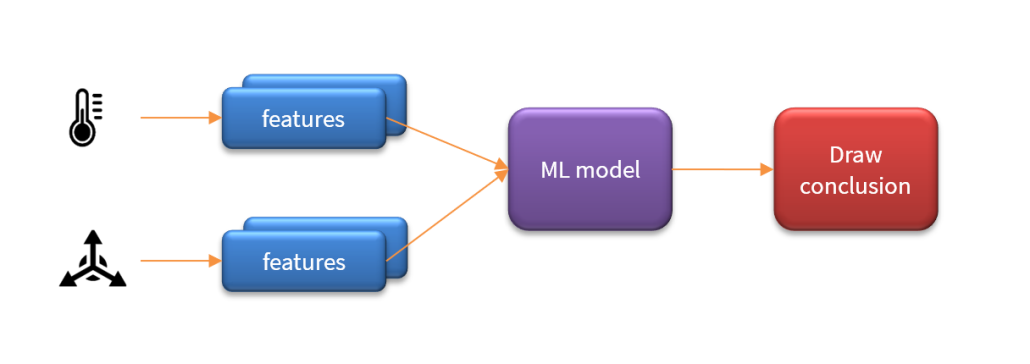
An ML model is the resulting output or predicted result after training an algorithm on a various datasets. It typically uses various feature extraction algorithms (e.g. mean, standard deviation and correlation) during the training period in order to extract features of interest for the ML model. The resulting model represents the learned patterns, parameters, or rules that can be used to make predictions on new data.
A key point to realise here, is that unlike algorithms based on predefined rules and mathematical concepts, how the ML model reaches its result remains an enigma, and is the primary reason why they shouldn’t be allowed to operate without any scrutiny on critical processes. As such, AI systems are energy constrained Boltzmann machine models, as the model is trained on data.
In many AIoT applications, Kalman based sensor fusion is typically used for feeding the ML model with high quality features of the underlying process, thus significantly improving the accuracy of the AI system.
How Algorithms and DLN/ML Models Interact
A model provides the capability to make decisions based on input data. It can recognize patterns, make predictions, and adapt to new information. Essentially, a model simulates cognitive functions that are typically associated with human thinking, such as dealing with ambiguity and uncertainty, but as discussed in a previous article, AI does not have any common sense, as it has no understanding of the underlying data or process that it is modelling.
On the other hand, an algorithm is a set of defined instructions or a mathematical recipe. It is a rules based step-by-step procedure used for calculations, data processing, and automated reasoning tasks. Algorithms are the backbone of software and can solve a wide range of problems by following their defined logic.
However, not all functions are computable. This means that there are certain problems for which no algorithm can be formulated to provide a solution. These are referred to as non-computable functions. In such cases, even the most advanced algorithms cannot determine an outcome, highlighting a fundamental limitation in computational theory.
Human Intelligence and Digital Intelligence
In the field of computation, it is essential to differentiate between traditional algorithms and machine learning models. An algorithm is a direct output of human intelligence, crafted through logical reasoning and problem-solving techniques. It represents a set of predefined instructions designed to solve specific problems. The human mind formulates these steps to ensure a consistent and accurate outcome.
In contrast, a trained machine learning (ML) model is the product of digital intelligence. While algorithms underpin the model’s structure, the true power of an ML model arises through its capacity to learn and adapt from new training data. This process involves iteratively adjusting parameters to optimize performance in tasks like prediction, classification, or decision-making. In this sense, the model evolves beyond its initial algorithmic foundation, generating insights and results that may not be directly encoded by human logic.
“An algorithm is a direct manifestation of human intelligence, designed through logic, reasoning, and problem-solving techniques. On the other hand, a trained machine learning model represents the outcome of digital intelligence, which evolves through the iterative processing of data.”
The convergence of these two forms of intelligence—human and digital—marks a significant shift in computational systems. Algorithms, though foundational, are static and require manual updates. Machine learning models, by contrast, learn from experience, dynamically evolving with each new piece of training data. This shift positions ML models as more flexible and adaptive tools for solving complex problems where human-defined rules may fall short.
The distinction between human-driven algorithms and data-driven machine learning models emphasizes the growing role of adaptive systems in areas such as autonomous driving, personalized medicine, and financial forecasting. As machine learning continues to evolve, the boundaries between explicit programming and emergent behavior will continue to blur, paving the way for systems capable of independent learning and decision-making.
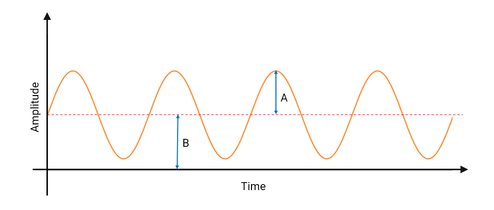
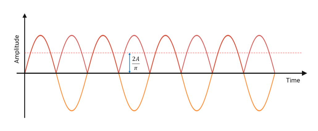
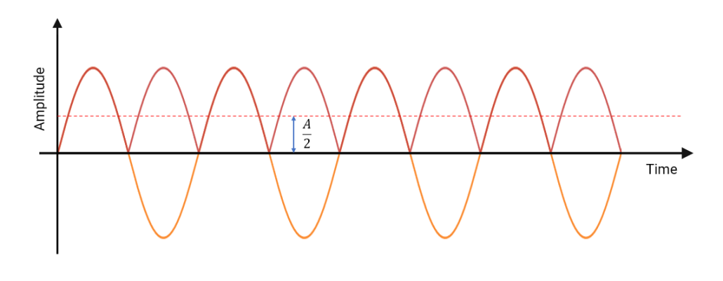
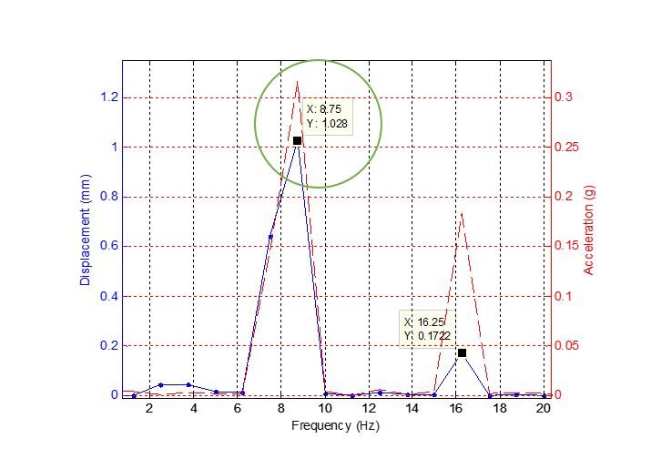
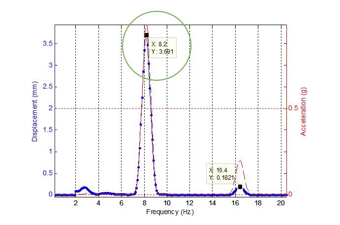
Low-Pass Filter and CNN for Classifying Periodic Signals
Both a Low-Pass Filter (LPF) and a Convolutional Neural Network (CNN) can be employed to handle periodic signals, but their approaches and purposes differ fundamentally.
Low-Pass Filter (LPF)
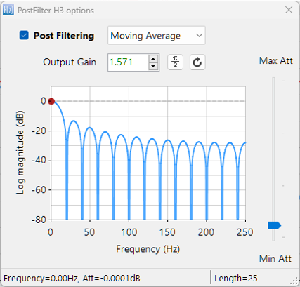
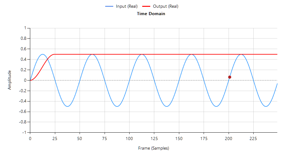
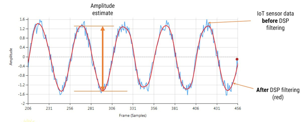
A Low-Pass Filter is an algorithm designed to attenuate the high-frequency components of a signal while allowing the low-frequency components to pass. Its primary use is to filter or clean a signal rather than classify it. Applications of the LPF in AIoT, include removing glitches from sensor data or even cleaning up noise on a measured periodic signal prior to feature extraction and subsequent ML classification, leading to higher accuracy.
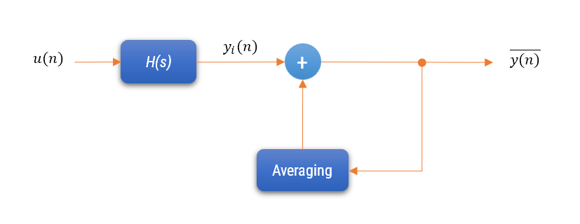
A practical IIR (infinite impulse response) digital filter used in both AIoT and IoT may be defined in terms of a finite number of poles \(p\) and zeros \(q\), as defined by the linear constant coefficient difference equation,
\(\displaystyle y(n)=\sum_{k=0}^{q}b_k x(n-k)-\sum_{k=1}^{p}a_ky(n-k) \)
where, \(a_k\) and \(b_k\) are the filter’s denominator and numerator polynomial coefficients, who’s roots are equal to the filter’s poles and zeros respectively. LPF filter can used for all types of signals, not just periodic signals. However, for this article we limit the discussion to periodic signals.
Limitations for Classification
While an LPF can enhance a periodic signal by reducing high-frequency noise, it does not classify the signal. It merely transforms the input based on fixed mathematical operations, with no ability to learn from data or adapt its behaviour.
Convolutional Neural Network (CNN)
A Convolutional Neural Network (CNN) is a machine learning model designed to recognize patterns in data by learning from training examples. It can be trained to classify periodic signals by learning distinctive features in the signal’s structure.
Operation
The CNN applies a series of convolution operations:
\(\displaystyle S(i,j) = (I * K)(i,j) = \sum_m \sum_n I(m,n) K(i-m, j-n) \)
where \(I\) is the input signal, \(K\)is the kernel, and \(S(i,j)\) is the resulting feature map.
Classification
Unlike the LPF, the CNN is capable of learning to classify different periodic signals through training. The learned filters allow the network to distinguish between signals based on the periodic features it identifies.
Extraction vs Learned feature
- Low-Pass Filter: Performs a deterministic operation that modifies the signal but cannot classify it.
- CNN: Learns from data and can classify periodic signals by recognizing their features.
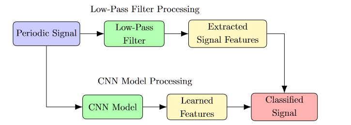
In conclusion, while a Low-Pass Filter may assist in signal preprocessing, a CNN is required for the task of classifying signals.
Adaptive Low-Pass Filters
An adaptive low-pass filter (LPF), such as those based on the Least Mean Squares (LMS) algorithm, introduces several key features and benefits compared to a traditional, static LPF:
- Dynamic Adaptability: Adaptive LPFs adjust their characteristics in response to variations in the input signal, allowing for real-time filtering of noise or unwanted frequencies, especially in non-stationary signals.
- Error Minimization: These filters utilize a feedback mechanism to minimize the difference (error) between the desired output and the actual output. The filter coefficients are continuously updated based on this error, enhancing the filter’s adaptability to changing signal conditions.
- Improved Performance in Noisy Environments: Adaptive LPFs effectively reduce noise by optimizing signal quality, which is particularly valuable in applications like audio processing, telecommunications, and biomedical signal processing where signal characteristics can fluctuate.
- Applications in Real-Time Systems: The adaptability of these filters makes them suitable for real-time systems, such as echo cancellation in telecommunication, where the noise characteristics may vary dynamically, ensuring consistent performance over time.
- Computational Complexity: While adaptive filters provide significant advantages, they also come with increased computational complexity due to the need for constant updates to the filter coefficients, which can be a concern in systems with limited processing capabilities.
In summary, using an adaptive LPF enhances the filter’s ability to handle varying signal conditions effectively, making it particularly valuable in applications requiring real-time signal processing, thus improving overall performance and robustness against noise and interference.
Adaptive low-pass filter (LPF) differs significantly from a traditional LPF in terms of feature extraction and learning capabilities.
Feature Extraction vs. Feature Learning
- Traditional LPF: This filter focuses on extracting specific frequency components from a signal by applying fixed coefficients determined by the filter design, which remain constant during operation. As a result, it extracts features based on pre-defined criteria.
- Adaptive LPF: Utilizes algorithms like the Least Mean Squares (LMS) to adjust its filter coefficients in real-time based on the input signal characteristics. This enables the adaptive LPF to extract features that dynamically correspond to changing signal conditions, but it does not learn features in the same manner as a neural network.
Comparison with CNNs
- Convolutional Neural Networks (CNNs): CNNs are designed to learn features from data through multiple layers, allowing them to automatically extract high-level features from raw inputs. Unlike traditional LPFs, CNNs perform feature learning, adapting to the input data through training on labeled datasets.
- While adaptive LPFs adjust their response based on signal changes, they do not perform feature learning like CNNs. They can optimize their filter characteristics based on feedback but lack the hierarchical feature learning approach present in CNNs.
Adaptive LPFs can extract features based on the immediate conditions of the signal; however, they do not ‘learn’ features in the same way that CNNs do. Instead, adaptive LPFs optimize the extraction process in real-time, making them effective in environments where signal characteristics vary.
Comparison of Adaptive Low-Pass Filters and Convolutional Neural Networks
Adaptive low-pass filters (LPFs), such as those using the Least Mean Squares (LMS) algorithm, exhibit several similarities with convolutional neural networks (CNNs) regarding their operational principles and learning mechanisms.
- Adaptive Coefficients: Adaptive LPFs modify their coefficients based on the input signal, similar to how CNNs adjust their weights during training to minimize loss on a dataset.
- Supervised Learning: Both systems can be trained using labeled data to optimize performance. Adaptive filters adjust based on real-time feedback while CNNs learn complex patterns through multiple iterations.
- Feature Extraction: Adaptive LPFs extract relevant features dynamically, while CNNs automatically learn to identify hierarchical features through their architecture.
- Learning Methodology: Adaptive LPFs adjust their parameters based on incoming data but do not learn complex representations as CNNs do. CNNs can learn multiple levels of abstraction through backpropagation.
- Structure and Complexity: CNNs consist of multiple layers, allowing them to learn intricate patterns, whereas adaptive LPFs typically operate with a single, simpler structure focused on modifying coefficients.
Items 1,2 and 3 are similar, but item 4 and 5 are different.
While adaptive LPFs and CNNs share similarities in their adaptive behaviors and feature extraction capabilities, they fundamentally differ in methodologies and complexities. Adaptive LPFs do not fully replicate the intricate learning capabilities of CNNs, though both aim to improve task performance through adaptation.
Comparison of Adaptive LPFs and CNNs
- Order of the Filter: The order of an adaptive low-pass filter (LPF) determines its ability to capture and process complex signal characteristics. A higher-order filter can approximate a more complex frequency response, allowing it to better handle diverse signal patterns, similar to how a deeper convolutional neural network (CNN) can learn more complex representations.
- Learning Capabilities: While both CNNs and adaptive LPFs adjust their parameters based on input, CNNs inherently possess a more advanced learning capability through multiple layers, each designed to extract different levels of abstraction from the data. This allows CNNs to learn hierarchical feature representations effectively. In contrast, increasing the order of an adaptive LPF can enhance its feature extraction capabilities, but it still lacks the sophisticated learning mechanisms that CNNs implement, such as backpropagation and convolutional operations.
- Complex Features: CNNs excel in extracting spatial hierarchies in data (e.g., images) by applying filters across multiple layers, progressively identifying edges, shapes, and more abstract features. Adaptive LPFs, when designed with a higher order, can capture complex signal behaviours, but their ability to generalize or learn from large datasets is limited compared to CNNs.
While increasing the order of an adaptive LPF can enhance its performance in signal processing, it does not equate to the deep learning capabilities of CNNs. CNNs utilize their layered architecture to learn complex features in a more robust and generalized manner, making them more suitable for tasks like image recognition and classification.
Parameter Estimation
Parameter estimation plays a crucial role in both traditional algorithmic processes and machine learning. It involves determining the best parameters for a given model based on observed data.
Algorithmic Parameter Estimation
In traditional algorithmic contexts, parameter estimation involves using specific algorithms to find optimal parameters for mathematical models. Key methods include:
Least Squares Estimation (LSE)
This method minimizes the sum of the squared differences between observed and predicted values. The parameter estimation is given by:
\(\displaystyle\hat{\theta} = \arg \min_{\theta} \sum_{i=1}^n (y_i – f(x_i; \theta))^2 \)
where \(\hat{\theta}\) denotes the estimated parameters. this concept is is central to Kalman filtering, whereby a state-space model of the process to be modelled uses the state estimates (i.e. the parameters of interest) to perform the prediction. The Kalman update equations attempt to minimise the error between the model output and the observed data in a least squares sense on a sample-by-sample basis.
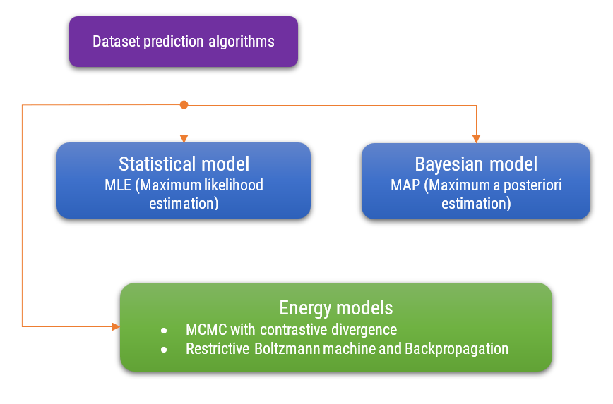
Maximum Likelihood Estimation (MLE)
MLE estimates parameters by maximizing the likelihood function, which reflects the probability of the observed data under the model parameters:
\(\displaystyle\hat{\theta} = \arg \max_{\theta} L(\theta; \text{data}) \)
where \(L(\theta; \text{data})\) represents the likelihood function.
Parameter Estimation in Machine Learning
In machine learning, parameter estimation is integral to model training and involves iterative optimization techniques. Examples include:
Training Neural Networks
Parameters such as weights and biases are estimated using gradient-based optimization methods, typically through:
\(\displaystyle\theta_{n+1} = \theta_n – \alpha \nabla_{\theta} L(\theta_n)\)
where \(\theta_n\) represents the parameters at iteration \(n\), \(\alpha\) is the learning rate, and \(L(\theta)\) is the loss function.
Bayesian Parameter Estimation
In Bayesian methods, parameters are estimated based on posterior distributions that combine prior beliefs with observed data:
\(\displaystyle p(\theta | \text{data}) \propto p(\text{data} | \theta) \cdot p(\theta)\)
where \(p(\theta | \text{data})\) is the posterior distribution.
In both traditional algorithms and machine learning contexts, the aim is to find the optimal parameters that best fit the model to the observed data.
Key Takeaways
Many people frequently refer to an ML model as an algorithm. This is incorrect, although the two terms are very closely related. An algorithm is a direct output of human intelligence, crafted through logical reasoning and problem-solving techniques. It represents a set of predefined instructions or a mathematical recipe designed to solve specific problems. The human mind formulates these steps to ensure a consistent and accurate outcome. In contrast, a trained machine learning (ML) model is the product of digital intelligence that uses algorithms and datasets to construct an ML model.
A key takeaway is that algorithms are based on predefined rules and mathematical concepts, whereas AI systems are energy constrained Boltzmann machine models, as the model is trained on data. As such, how an ML model reaches its result remains an enigma, and is the primary reason why they shouldn’t be allowed to operate without any scrutiny on critical processes.