From lithography machines to medical instruments, real-world edge systems demand deterministic behaviour, reliable sensor interpretation, and carefully engineered algorithms that go far beyond simply training an AI model.
Artificial Intelligence or AI has been glorified as the future of automation, often portrayed as the ultimate solution for efficiency, decision-making, and innovation across industries. It is marketed as a transformative technology for everything from healthcare and finance to autonomous systems and industrial processes.
In practice, this narrative does not reflect present reality, as AI in its current form remains too limited to be relied upon for mission-critical applications that require deterministic behaviour, such as those stipulated by ISO/IEC standards. Although AI performs impressively in controlled settings, it often struggles when exposed to the complexity, variability and unpredictability of real-world environments — particularly when those conditions fall outside the assumptions used to train the model.
This degradation in performance occurs because AI lacks common sense reasoning and struggles with real-world subtlety, i.e. it does not understand the real world in the same way that humans do. Trained largely on synthetic or otherwise limited datasets, it has no intrinsic grasp of the physical or situational subtleties present in operational environments. When real-world conditions differ from those seen during training, AI systems often misinterpret context, leading to unreliable or misleading outcomes — an unacceptable limitation for any mission-critical application.
What is a mission-critical application?
An application is classed as mission-critical when results must be delivered predictably, repeatably and within guaranteed timing constraints defined by system and stakeholder requirements. In many operational environments, unreliable or delayed behaviour can lead directly to financial loss, disrupted processes or regulatory non-compliance. In embedded edge systems (e.g. semiconductor lithography machines, factory automation, medical instruments and logistics automation), algorithms interact directly with physical processes under strict constraints such as bounded latency, limited computational resources, low power consumption and long-term reliability, while often needing to comply with IEC/ISO standards.
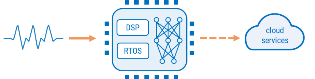
At the heart of these systems are physical measurements, i.e. sensors that produce signals that reflect real-world processes, but are often corrupted by noise, interference and environmental disturbances. This broader challenge is increasingly discussed under the banner of Physical AI — intelligent systems that perceive, reason and act within the physical world through sensors, signals and real-time control. Achieving this in practice requires the integration of deterministic digital signal processing (DSP) algorithms, machine learning (ML) and embedded systems design, forming the basis of Real-Time Edge Intelligence (RTEI).
Intelligent machines existed long before AI
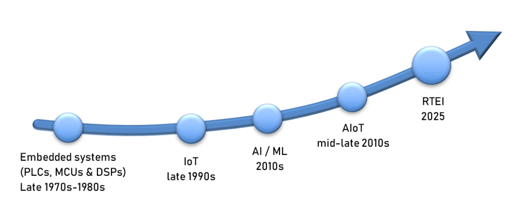
The idea of embedding intelligence into machines predates modern AI by decades. Early automation systems implemented rules‑based behaviour using mechanical logic and later electromechanical control systems. However, with the development of electronics, these concepts evolved into embedded systems built on PLCs, microcontrollers (MCUs) and later digital signal processors (DSPs), allowing complex signal analysis and control algorithms to be implemented in software while maintaining robust deterministic behaviour.
Figure 1: Evolution of intelligent systems. From embedded systems to connected IoT platforms and modern edge devices combining DSP and ML techniques.
The rise of IoT
As sensing technologies became cheaper and connectivity expanded, embedded devices increasingly became networked, leading to the Internet of Things (IoT). In many architectures, devices primarily act as data forwarders, streaming sensor measurements to cloud infrastructure where ML models perform analysis.
While this approach enables powerful functionality, it also introduces limitations such as network latency, bandwidth consumption and dependence on continuous connectivity. For many real‑world systems, intelligence must therefore move closer to the data source.
The challenge of real‑world sensor data
Real-world sensor data are rarely clean, as the signals are affected by measurement noise, powerline interference and environmental disturbances. As such, extracting meaningful information from these measurements has traditionally relied on signal processing techniques, implemented either using analog electronics or digitally using a DSP or microcontroller. These techniques perform tasks such as filtering, spectral analysis and feature extraction. Filtering removes noise, spectral analysis reveals hidden patterns and feature extraction transforms raw measurements into structured information describing the underlying system behaviour. These deterministic methods make signal interpretation predictable and verifiable.
The Evolution from Edge AI to RTEI
ML models operate most effectively on a few well‑designed features based on the physics of the sensor data. In order to facilitate this, DSP algorithms (designed using human intelligence) are a fundamental pre-step for signal enhancement and feature extraction, such that the ML model can perform its classification task based on high-quality feature data. It is this combination that can provide high classification accuracy, even when conditions slightly deviate from the original training datasets.
Figure 2: RTEI architecture. Sensor measurements are processed through deterministic DSP algorithms to extract meaningful features for ML inference on the edge device. An optional cloud connection provides secondary services such as access to a data lake and device management.
As such, engineers are increasingly adopting architectures in which DSP, ML and the embedded computing platform (e.g., Arm Cortex processors with hardware support for DSP and ML workloads) are developed together, while remaining aligned with stakeholder requirements and relevant IEC/ISO compliance standards. This augmented approach improves reliability while ensuring long-term robustness across a wide range of edge applications.
RTEI Solutions Handbook
The architectural principles behind Real-Time Edge Intelligence (RTEI), including practical DSP techniques, embedded implementation strategies and real-world case studies, are explored in detail in RTEI solutions handbook, which may be purchased directly from ASN.
Sanjeev is a RTEI (Real-Time Edge Intelligence) visionary and expert in signals and systems with a track record of successfully developing over 26 commercial products. He is a Distinguished Arm Ambassador and advises top international blue chip companies on their AIoT/RTEI solutions and strategies for I5.0, telemedicine, smart healthcare, smart grids and smart buildings.
https://www.advsolned.com/wp-content/uploads/2026/03/Sanjeev_rteibook-e1773052346437.png6081081Dr. Sanjeev Sarpalhttps://www.advsolned.com/wp-content/uploads/2021/07/asn_logo_red_met_tekst_helder-e1755353934770.pngDr. Sanjeev Sarpal2026-03-09 11:25:592026-06-22 13:17:03Why Intelligent Edge Systems Need More Than Just AI
Over the past 40 years, I’ve worked with a wide range of microcontrollers and DSPs across industries—from biomedical systems and industrial control to radar and audio processing. What follows is not theory—it’s a reflection based on firsthand experience with many of the chips and platforms that have shaped the embedded world as we know it.
Before the Age of General-Purpose DSPs
In the early 1980s, Digital Signal Processing (DSP) was often too demanding for microprocessors, which lacked the speed and specialised instruction sets. To address this, manufacturers developed dedicated hardware accelerators—custom ICs built to perform tasks such as Fast Fourier Transforms (FFT), digital filtering, and modulation. Companies such as TRW LSI Products, Harris Semiconductor and even Intel offered function-specific chips that could be dropped into hardware designs to offload processing from the main CPU. These chips laid the groundwork for programmable DSPs, which would later unify these capabilities into a single, software-controlled processor—offering far greater flexibility and reusability.
The Three Titans of Classic DSP: TI, Analog Devices and Motorola
Back in the golden age of classic DSPs, three companies stood out: Texas Instruments, Analog Devices, and Motorola. Each brought its own innovations, architectures, and ecosystems that defined digital signal processing for decades.
Texas Instruments (TI) took the lead with its TMS320 family. Initially introduced in 1983, the fixed-point TMS32010 was one of the first general-purpose DSPs on the market. TI’s later C2000 series brought DSP-like performance to microcontrollers—making it a popular choice for motor control and industrial automation. But it was the TMS320C6000 series, launched in the late 1990s, that truly set a new benchmark. These VLIW (Very Long Instruction Word) DSPs—such as the C62x (fixed-point) and C67x (floating-point)—enabled complex signal analysis, control, and real-time processing with high instruction throughput.Later multicore versions like the C6474 scaled this up with three high-performance DSP cores on a single chip. Some designs even scaled to six cores in custom implementations. These chips made it possible to perform real-time control, sensor fusion, and high-throughput signal analysis in a way that felt almost futuristic —achieving over 28,000 MIPS!
TI also addressed ultra-low-power use cases with the C55x series—a fixed-point DSP line optimised for battery-powered audio and telecommunication applications. Whether for performance or power efficiency, TI had an answer across the spectrum.
Analog Devices (ADI) also played a central role in shaping DSP. Their SHARC and TigerSHARC families offered high-performance floating-point computation, making them a favourite in professional audio, instrumentation, and aerospace applications. Equally important was the Blackfin family—a fixed-point, 16/32-bit hybrid architecture introduced in the early 2000s. Blackfin was optimised for embedded multimedia and signal processing tasks, combining DSP capability with control-oriented features like MMUs, timers, and flexible I/O. ADI offered excellent tools, tight integration with analog components, and very strong real-time performance for demanding applications.
Motorola, meanwhile, contributed both microcontroller and DSP innovations. The legendary 68000, launched in 1979, wasn’t strictly a DSP, but it offered 32-bit general-purpose performance that was far ahead of its time. It was widely adopted in embedded control systems and even some signal processing applications—powering everything from defence platforms to the Commodore Amiga. Motorola also developed a dedicated line of DSPs in the 56000 family, which gained a following in telecommunications and audio. Eventually, Motorola spun off its semiconductor business as Freescale, and later moved to PowerPC architectures. Still, its legacy in early DSP computing remains significant.
Collectively, these three vendors established the blueprint for programmable signal processing—offering both fixed-point and floating-point variants, with increasing performance, integration, and software support over time. Their contributions laid the groundwork for today’s hybrid processors, SoCs, and enhanced microcontrollers.
Enter Microchip’s dsPIC: A Different Kind of DSP
When Microchip launched the dsPIC series in 2001, it was a radical departure from the classic DSP playbook. Instead of focusing on high-performance signal processing, Microchip blended DSP-like instructions into a 16-bit microcontroller core—creating a hybrid that prioritised real-time control, affordability, and embedded peripherals all-in-one. This unorthodox approach defied convention, yet proved surprisingly effective in areas such as motor control and power electronics.
In 2007, Microchip introduced the PIC32, a 32-bit fixed-point MIPS architecture intended to compete with Arm-based microcontrollers. Floating-point support only arrived in PIC32MZ devices in 2013, which still retained the MIPS lineage. By then, the industry had largely moved on. After acquiring Atmel in 2016, Microchip began transitioning toward Arm-based designs—but found themselves playing catch-up. STMicroelectronics, NXP, and others had already embraced Arm more than a decade earlier.
Hitachi and the SH Architecture
Another important player in the 1990s was Hitachi, whose SuperH (SH) family of microcontrollers gained traction in both consumer electronics and automotive systems. The SH architecture offered a compact 32-bit RISC instruction set and DSP-like instructions, making it well-suited for signal processing tasks without the complexity of a full DSP.
The SH-2, in particular, was developed for motor control and stood out for its high performance and nicely designed 32-bit architecture. It was backed by a professional-grade toolchain—more expensive than Microchip’s offerings, and far more capable. While Microchip’s later dsPIC family also targeted fixed-point DSP applications, it was positioned more toward the hobbyist and cost-sensitive market. In contrast, the SH-2 catered to industrial and automotive use cases that demanded greater precision, performance, and software maturity.
The SH line powered everything from set-top boxes and printers to game consoles, with the SH-2 used in the Sega Saturn and the more powerful SH-4 driving the Sega Dreamcast. After merging with Mitsubishi’s semiconductor division to form Renesas in 2003, the SH series continued for a while but was gradually replaced by newer architectures such as RX and eventually Arm-based cores. Nonetheless, the SH family remains a fascinating example of early DSP-capable microcontrollers.
How Arm Processors Changed the Game
The real turning point for Arm came in 1995, when they secured a major contract with Nokia. At the time, Nokia was searching for a low-power processor for its mobile phones—something that could offer signal processing without the power drain of conventional DSPs.
Arm responded with the Thumb instruction set—a compact 16-bit format that dramatically reduced code size while preserving much of the performance of 32-bit Arm instructions. Later, Thumb-2 extended this approach with mixed 16/32-bit support, enabling DSP-like functionality within a power-efficient and compact silicon footprint. It was a game-changer.
However, what truly propelled Arm forward was its strategy and licensing model. Rather than manufacturing chips themselves, Arm licensed its processor IP to silicon vendors—forming deep partnerships with companies such as STMicroelectronics, NXP, Texas Instruments, and Analog Devices. These vendors integrated Arm cores into their own SoCs, often alongside analog front ends, accelerators, or even DSP blocks. The result was a wave of highly optimised, application-specific devices built atop a shared architecture.
A key milestone came with Broadcom’s adoption of the Cortex-A family, which powered the first Raspberry Pi. The Pi’s success brought Arm processors into education, prototyping, and hobbyist markets—seeding a new generation of developers trained on Arm platforms.
Combined with a robust ecosystem of compilers, development tools, and middleware, Arm’s architectural dominance spread rapidly across consumer, industrial, and IoT domains.
The Emergence of the Enhanced Microcontroller
Today’s microcontrollers are far more than just control engines. Many now include SIMD instructions, DSP acceleration, advanced timers, cryptographic modules, and hardware-based security. This gives rise to what might be called the enhanced microcontroller—a class of devices that blur the line between DSPs and MCUs.
Today’s microcontrollers are no longer just simple control devices. Many now include SIMD instructions, DSP acceleration, and hardware-based security. This gives rise to what we can call the enhanced microcontroller—a hybrid class that combines:
General-purpose control and peripheral integration
DSP capabilities for signal conditioning and real-time analysis
Hardware security features such as TrustZone
Low power consumption for battery-powered and IoT systems
Affordable pricing for mass deployment
STMicroelectronics’ STM32 family—based on Cortex-M4 and M7 cores—is a textbook example. These microcontrollers can handle filtering, FFTs, and real-time signal analysis with ease, all while supporting familiar C-based toolchains and low-power sleep modes. They may not match a high-end floating-point DSP in every respect, but they strike an ideal balance for most embedded applications.
Arm Helium: Specialised Edge Hardware Acceleration
Arm Helium—also known as the Armv8.1-M Scalable Vector Extension (MVE)—takes this trend a step further. Designed for edge AI, Helium allows microcontrollers to perform complex filtering, sensor fusion, and even neural inference tasks with impressive efficiency.
The Cortex-M52 captures the essence of this shift—bringing DSP, general-purpose control, security, and low-power performance together into a single core. It introduces Arm TrustZone for embedded security, supports Helium acceleration, and enables localised processing of tasks that once required external compute or specialised DSPs.
Many new Helium-based MCUs also leverage TSMC’s 22nm ultra-low-power process, delivering up to 50% power savings over 40nm chips. This makes edge intelligence viable even in battery- or solar-powered deployments, with no compromise on performance.
It’s Not Just the Hardware—It’s the Ecosystem
Arm’s success is also rooted in the richness of its ecosystem. Developers benefit from mature toolchains, CMSIS-DSP libraries, trusted third-party support, and a wide community of contributors.
This infrastructure allows engineers to focus on solving domain-specific problems rather than wrestling with the underlying hardware. Thanks to tools from ASN, Qeexo, Mathworks and Edge Impulse even sophisticated algorithms—such as biomedical filters, IoT sensor cleaning filters, and predictive maintenance monitors—can now be designed, validated, and deployed as efficient C code within minutes, without requiring deep DSP expertise.
Arm’s ecosystem lowers the entry barrier while raising the ceiling, enabling individual developers and small teams to compete with traditional DSP engineering departments. It’s this accessibility and scalability that makes the platform so compelling for modern embedded development.
Enter the Market Disruptor: Espressif Semiconductor
While much of the evolution in embedded DSP has been driven by microcontrollers based on Arm-Cortex cores from vendors such as STMicroelectronics, Texas Instruments, Analog Devices and NXP, a disruptive force entered the scene in 2016 with the launch of Espressif Semiconductor’s ESP32-WROOM-32.
Based on dual-core Xtensa® 32-bit LX6 processors, the original ESP32 combines integrated Wi-Fi and Bluetooth with a hardware single-precision floating-point unit (FPU) and DSP-style instructions such as multiply-accumulate and saturation arithmetic. Despite lacking hardware support for division and square root, its real-world floating-point performance is often comparable to an Arm Cortex-M4F, thanks to its 240 MHz clock and efficient memory architecture.
Originally aimed at wireless control applications, the ESP32 quickly gained traction for low-cost edge processing tasks—including audio filtering, FFT analysis, and real-time control. Espressif’s open SDK and active global community positioned it as the go-to resource for hobbyists, start-ups, and even commercial IoT products.
While it lacks the advanced DSP acceleration of Arm Helium or the precision of high-end floating-point DSPs, the ESP32’s exceptional cost-to-performance ratio has democratised edge intelligence. It has showed the world that embedded DSP doesn’t have to be expensive or exclusive.
Where Do We Stand Now?
DSP has not disappeared—it has evolved. What was once the domain of dedicated chips has become a fundamental capability, embedded across a wide range of computing platforms. From soft DSP cores in FPGAs to integrated signal processing units in SoCs, and now to scalable vector extensions within microcontrollers, the function of DSP is alive and well—although the form has changed.
Specialist chips, such as those from Texas Instruments or Analog Devices, have not vanished. Many are now integrated into SoCs—handling radar, video, and high-performance industrial tasks in highly integrated systems. The IWR6834 mmwave radar SoC from TI is a perfect example of this convergence: a C674x floating point DSP, two Arm Cortex-R4 processors, communication channels, memory, RF frontend, and antennas all in one compact, high-performance chip. Newer flavours of the SoC, include an AI engine for micro-doppler pattern classification. All of which can be inferenced at the edge in real-time!
However, for most embedded applications, enhanced microcontrollers based on Arm processors now deliver the best balance of performance, power, and price. With integrated support for signal processing, connectivity, security, and energy efficiency—all within a mature ecosystem—they have become the logical choice for the next generation of intelligent edge devices.
Across the Cortex-M family, options like the M4 and M7 provide a strong foundation for signal processing in real-time control applications. The Helium-enabled M55, M85, and most recently the M52, take this further—offering vectorised DSP acceleration, better energy efficiency, and increasingly robust security features.
The Cortex-M52 in particular captures the essence of this evolution. It unifies three essential capabilities for Edge AI into one compact, low-power device:
DSP/AI functionality for signal processing algorithms, such as filtering and feature extraction, and running ML models
Low power consumption to enable battery or energy-harvesting applications
Hardware-based security, including Arm TrustZone, to safeguard code and data
This convergence enables true Real-Time Edge Intelligence (RTEI)—where signals are captured, interpreted, and acted upon locally, without relying on cloud infrastructure or external accelerators. Tasks such as biomedical filtering, sensor fusion, anomaly detection, and embedded inference can now be performed directly at the edge, at a fraction of the power and cost of what was previous required.
And with newer devices manufactured on advanced low-power nodes—such as TSMC’s 22nm process—power consumption is reduced by up to 50% compared to older 40nm designs. This makes the deployment of smart, responsive, and secure edge systems more sustainable and scalable than ever before.
And today, over 90% of all microcontrollers use an Arm core, which is a testament to Arm’s rich ecosystem and proven technologies.
This is not just a shift in hardware—it’s a redefinition of where and how computing happens in the embedded world of 2025 and beyond. It happens in real time, at the edge.
The RTEI solutions handbook covers this exciting technological journey in more detail and is available directly from ASN.
Sanjeev is a RTEI (Real-Time Edge Intelligence) visionary and expert in signals and systems with a track record of successfully developing over 26 commercial products. He is a Distinguished Arm Ambassador and advises top international blue chip companies on their AIoT/RTEI solutions and strategies for I5.0, telemedicine, smart healthcare, smart grids and smart buildings.
https://www.advsolned.com/wp-content/uploads/2025/07/superhuman.png10241024Dr. Sanjeev Sarpalhttps://www.advsolned.com/wp-content/uploads/2021/07/asn_logo_red_met_tekst_helder-e1755353934770.pngDr. Sanjeev Sarpal2025-07-07 15:48:472026-04-06 12:35:09The Birth of Real-Time Edge Intelligence: When DSP and AI Met the Arm Processor
In our age of AI, IoT, and real-time signal processing, it’s tempting to believe that algorithmic thinking is a modern invention. But over 1,100 years ago, in the heart of the Islamic Golden Age, two extraordinary thinkers were already shaping what we now call systems engineering: Muḥammad ibn Mūsā al-Khwārizmī and Yaḥyā ibn ʻAdī al-Kindī.
Their brilliance wasn’t just in what they knew—it was in how they thought.
The Power of Critical Thinking
Al-Khwārizmī and Al-Kindī lived in a time when knowledge was unified. Mathematics, philosophy, astronomy, and medicine were seen as part of a single, coherent worldview. This intellectual breadth allowed them to see connections others missed.
In some ways, generative AI attempts to mimic this cross-disciplinary reach—drawing associations across vast domains with billions of model parameters. But unlike Al-Kindī and Al-Khwārizmī, it operates without commonsense, without understanding, and without true context. This alone makes AI fundamentally inferior to the critical thinking of these scholars. Their minds weren’t just expansive—they were disciplined, purposeful, and deeply structured.
They also had something rare today: time. Freedom from the pressure to publish or the noise of constant alerts, they dedicated themselves to real understanding. Without emails, 24hour news feeds, or KPIs pulling at their attention, they achieved the kind of clarity that produced lasting contributions to mathematics, science, and cryptography—many of which still shape our world today.
Just as the Latinized name of Al-Khwārizmī gave rise to the word algorithm, the idea behind algorithms—structured procedures for solving problems—is far older and more global. Across different civilizations, these ideas took root in unique yet strikingly similar ways.
In classical Tamil, the word சூத்திரம் (sūthiram) has long referred to concise formulas or rules. Found in ancient grammar, mathematics, and philosophy, a suthiram was a compact, logical step—an algorithm in spirit. Tamil arithmetic manuscripts used them to express procedures for multiplication and permutations, echoing the same structured problem-solving seen in other cultures.
Even today, Tamil retains this legacy. In schools and textbooks, சூத்திரம் appears alongside the transliterated அல்காரிதம்—a reminder that algorithmic thinking has deep, indigenous roots. The algorithm is not a modern invention. It’s a universal pattern—and every culture has its own word for the thread.
This global legacy reminds us that algorithms were once tools of understanding, not just instruments of automation. If we are to use algorithms wisely today, we must restore that spirit: clear purpose, cultural context, and conscious design.
And Yet, Here We Are
Today, we automate decisions, and design systems that affect real lives. The legacy of Al-Khwārizmī and Al-Kindī challenges us to ask:
Are our algorithms truly serving people—or just chasing efficiency?
Nowhere is this more urgent than in AI. As we build increasingly powerful models, the temptation is to optimize for performance at all costs. But Al-Khwārizmī reminds us that an algorithm must be understandable. And Al-Kindī reminds us that it must serve human reason and values.
This is precisely why Real-Time Edge Intelligence (RTEI) is so important. RTEI combines human reasoning, grounded in deterministic DSP algorithms, with digital reasoning, driven by machine learning.
But there is a crucial difference: digital reasoning can hallucinate. It can invent patterns and correlations—what we sometimes call “creativity”—but it has no ethics, no intent, and no understanding. Human reasoning, on the other hand, brings structure, purpose, and responsibility.
RTEI is not just a technical fusion. It is a moral architecture: one that safeguards the unpredictability of AI with the reliability and interpretability of classical DSP. In a way, it echoes the very legacy of these scholars: logic and structure, guided by ethics and accountability.
A Principle That Still Applies in 2025
They remind us that clear, ethical, and deeply structured thinking transcends time.
This is where the classical principle of رفع الحرج (removal of hardship) becomes strikingly relevant. It wasn’t just about compassion—it was about reducing confusion and unnecessary complexity in systems.
RTEI carries this legacy forward: combining the reliability of DSP with the adaptability of ML to build systems that are powerful, yet clear and responsible. In a world where generative AI can hallucinate, we need that balance more than ever.
Sometimes, the most radical idea is to slow down and think like it’s the 9th century!
Sanjeev is a RTEI (Real-Time Edge Intelligence) visionary and expert in signals and systems with a track record of successfully developing over 26 commercial products. He is a Distinguished Arm Ambassador and advises top international blue chip companies on their AIoT/RTEI solutions and strategies for I5.0, telemedicine, smart healthcare, smart grids and smart buildings.
AI has been glorified as the future of automation, often portrayed as the ultimate solution for efficiency, decision-making, and innovation across industries. It has been marketed as an all-encompassing technology capable of transforming everything from healthcare and finance to autonomous systems and industrial processes.
In practice, this narrative does not match reality, as AI in its current form is too limited to be relied upon for mission-critical applications. While it has demonstrated some success in controlled settings, it struggles to adapt to real-world complexities and unpredictability. While tech giants celebrate cloud-trained AI models, these solutions typically fail spectacularly when deployed in dynamic, unpredictable environments. This is because AI lacks commonsense reasoning and struggles with real-world subtlety, i.e. it doesn’t understand the real world in the same way that humans do. It is typically trained on synthetic or limited datasets, which fail to fully capture the diverse and complex scenarios it is expected to handle. As a result, AI systems often misinterpret context, leading to unreliable or misleading outcomes in unpredictable operating environments.
The Consequences of AI’s Limitations
The lack of common sense of how the physical world works and limited training data is a fundamental limitation of AI systems. This can lead to costly failures, false predictions, and in worst cases, complete system breakdowns—making them unsuitable for environments where precision and reliability are paramount.
Another significant limitation, particularly for large-scale models like LLMs, is that AI models require powerful computing resources, making them inefficient for real-time, low-power edge applications. That being said, advancements in Nvidia’s latest chipsets, such as the Jetson Orin series are certainly helping bridge this gap by providing high-performance, power-efficient AI processing directly on edge devices.
While these new chipsets allow AI models to run locally and reduce reliance on cloud computing, AI in general still faces challenges such as excessive power consumption compared to deterministic DSP algorithm-based solutions, reliance on limited datasets, and a lack of explainability. These factors make AI unsuitable for industries requiring strict regulatory compliance and safety. While some smaller AI models can be optimised for edge deployment, many modern AI architectures remain computationally expensive and impractical for real-time, low-power edge applications.
Furthermore, most ML models rely on generalised feature extraction algorithms (mean, standard deviation, kurtosis, correlation etc) and are trained on limited, often unrealistic datasets. AI’s reasoning is entirely data-driven, meaning that we still don’t fully understand how the models work, making them very different from traditional DSP algorithms that use a mathematical recipe or a set of predefined rules. When faced with new, unseen conditions, AI often produces inaccurate or misleading results. In contrast, RTEI (Real-time Edge Intelligence) leverages DSP algorithms that are based on science, making them scientifically accurate and reliable in complex, real-world applications.
The AI Illusion: Why Traditional AI Fails at the Edge
Cloud-based AI solutions dominate today’s landscape because they require vast computational resources to function effectively. However, when deployed on edge devices with limited power and processing capacity, AI’s inefficiencies become apparent.
Predictive maintenance in industrial environments serves as a pertinent example. AI-based solutions are often promoted as game-changers, yet they struggle with a fundamental issue: the lack of real-world failure data. Most foremen and factory managers will not allow researchers to deliberately break machines for data collection, leading to AI models trained on synthetic or limited failure cases. As a consequence, this creates significant gaps in understanding of the normal and abnormal behaviour of the machine or process, leading to potential misdiagnoses and operational inefficiencies.
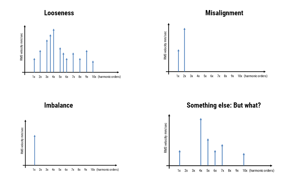
A more effective approach—Real-Time Edge Intelligence (RTEI)—combines DSP algorithms for feature extraction with ML models for classification. For example, in vibration analysis, DSP-based techniques can be used to generate harmonic fingerprints of velocity and displacement (feature extraction), which can be used to detect anomalies before they lead to system failure. These fingerprints or features are then fed into ML models for fault classification. This hybrid approach ensures accuracy and robustness, as DSP algorithms rely on physics and engineering principles (e.g. Fourier analysis, Kalman filtering) rather than data-driven learning.
RTEI: The Future of Edge Intelligence
RTEI (Real-time Edge Intelligence) represents a fundamental shift in AI for edge computing. By integrating real-time DSP algorithms with ML models, RTEI enhances accuracy, reliability, and computational efficiency. Unlike traditional AI, which operates on probabilistic reasoning, RTEI leverages fundamental scientific principles, making it more predictable and suited for mission-critical applications like autonomous vehicles, industrial automation, and medical diagnostics, where any misjudgements could have catastrophic consequences.
For Edge IoT to reach its true potential, intelligence must be embedded directly into devices. We are already seeing promising advancements—industrial-grade vibration analysis systems using real-time DSP algorithms to detect early signs of mechanical failure, and aircraft autopilot systems that rely on deterministic control algorithms rather than AI, ensuring mission-critical reliability in aviation, and self-driving cars that utilize LiDAR, cameras and other sensors to navigate autonomously without solely depending on AI-based decision-making. These systems prioritise reliability through scientifically proven methods rather than speculative, data-driven predictions.
As AI’s reasoning is fundamentally different to that of traditional DSP algorithms, a key point to realise here is that unlike DSP algorithms based on predefined rules and mathematical concepts (i.e. designed with human intelligence), how the AI reaches its result remains an enigma, and is the primary reason why they shouldn’t be allowed to operate without any scrutiny on critical processes.
RTEI enhances the overall solution by adapting its feature extraction algorithms to real-world variations, ensuring consistently high-quality data for AI classification. For example, when measuring analog sensor data using an ADC, temperature variations in the instrumentation electronics would cause the sampling rate to slightly vary. This variation would lead to a mismatch between the ideal model and real-world signal tendered to the classifier. As such, a conventional AI model would struggle, as these variations were probably not taken into account during the model’s training phase.
This is where DSP algorithms, such as a method that analyses timestamps or a Kalman filter can shine, as sampling rate variation can be taken into account in the estimation model. As such the DSP estimation algorithm can estimate the signal’s sampling rate in real-time and use this estimate to perform other operations required for the feature extraction operation. This ensures that only high-quality features are provided to the classifier in varying temperature environments—a very realistic scenario! Finally, it should be noted that this approach has the added advantage of requiring less ML training data, which expedites development and lowers project costs.
The Role of Arm Processors in RTEI
A major driving force behind this revolution is the Arm-based processor ecosystem. Unlike traditional cloud-based AI solutions, Arm Cortex processors (including the newer Arm Helium processors) provide a power-efficient way to run edge-optimized AI models in real-time. These processors are already at the core of smart sensors, embedded systems, and industrial automation, ensuring that AI-powered IoT devices can process and react instantly to changes in their environments.
Lockstep Processor Technology for Mission-Critical Systems
A fundamental aspect of mission-critical systems is Lockstep processor technology, which ensures redundancy and fault tolerance in real-time applications. Processors such as the Arm Cortex-R4 and Cortex-R5 are designed with lockstep functionality, where two identical processors run the same instructions simultaneously and compare results.
Lockstep technology is particularly useful for detecting hardware faults, which can arise from environmental influences, component ageing and external interference. For example, bit flips in memory can occur due to electromagnetic interference (EMI) from industrial machinery or power supply fluctuations, corrupting data memory and leading to algorithmic errors.
A key concept for dual-processor Lockstep processing is that it detects discrepancies but does not determine which processor is correct. Since both processors execute the same software, software bugs will appear identically on both, making lockstep ineffective for detecting programming errors. For true fault tolerance and error correction, a Triple Modular Redundancy (TMR) approach is often used, where three processors execute the same software, and a majority vote determines the correct outcome either per cycle or function.
ASIL Compliance and Automotive Safety
Lockstep technology is essential for Automotive Safety Integrity Level (ASIL) compliance, ensuring that automotive safety systems can detect and handle processor faults. For example, in an adaptive cruise control system, if a processor mismatch occurs, the system disengages cruise control rather than making an unsafe decision. This prioritisation of passenger safety over continuous operation is crucial for mission-critical applications.
For systems requiring the highest levels of reliability—such as flight control systems or nuclear power plants—TMR is employed to prevent a single fault from compromising the entire system.
Neoverse: High-Performance Edge Computing
Arm’s Neoverse architecture is a high-performance processor family designed for data centres, edge computing, and cloud infrastructure. Unlike Cortex processors, which are commonly used in mobile and embedded applications, Neoverse is optimized for scalability, power efficiency, and AI acceleration, making it well-suited for high-performance edge computing and is an interesting alternative to Nvidia’s Jetson Orin GPU series.
With advancements in Arm Cortex (especially Helium) and Neoverse architectures, developers can now deploy real-time AI workloads directly on edge devices, eliminating cloud dependencies. This means better security, reduced costs, and instant decision-making, all of which are essential for next-generation IoT applications.
Key takeway:The Evolution from AI to RTEI
Rather than dismissing AI’s role in edge applications, RTEI represents the next evolutionary step—one that acknowledges AI’s limitations and enhances its capabilities through deterministic DSP algorithms. Traditional AI struggles to generalize beyond pre-trained scenarios, lacks commonsense reasoning, and remains a black box in decision-making. These weaknesses make it ill-suited for dynamic, real-world applications.
The time has come to move beyond the assumption that cloud-trained AI can work everywhere. Instead, RTEI offers a hybrid intelligence system—combining the strengths of AI and DSP for real-time, reliable, and efficient edge intelligence.
By embedding intelligence directly into edge devices using Arm processors, lockstep technology, and deterministic DSP algorithms, we can build smarter, safer and more adaptable systems.
Sanjeev is a RTEI (Real-Time Edge Intelligence) visionary and expert in signals and systems with a track record of successfully developing over 26 commercial products. He is a Distinguished Arm Ambassador and advises top international blue chip companies on their AIoT/RTEI solutions and strategies for I5.0, telemedicine, smart healthcare, smart grids and smart buildings.
https://www.advsolned.com/wp-content/uploads/2024/10/robot_reading-scaled-e1729851827745.jpg7201080Dr. Sanjeev Sarpalhttps://www.advsolned.com/wp-content/uploads/2021/07/asn_logo_red_met_tekst_helder-e1755353934770.pngDr. Sanjeev Sarpal2025-01-31 15:05:132025-02-03 09:20:07Rethinking AI: Why Edge Intelligence must go beyond traditional ML
Generative AI (software capable of producing new content such as text, images, music or animations) has captured the public’s imagination. Many websites offer tools for creating playful visuals or novelty outputs with just a few clicks, but these entertainment-focused applications often fail to address the pressing, real-world demands of modern businesses.
While such generative technologies excel at creativity and rapidly prototyping ideas, Real-Time Edge Intelligence (RTEI) is positioned to have a far greater impact where it counts most, i.e. mission-critical operations. By processing data at the Edge and providing immediate insights, RTEI directly tackles key needs in manufacturing, healthcare, automotive, logistics, and other fields—scenarios in which split-second decisions and reliability are paramount.
Immediate Decision-Making
While generative AI excels at creative tasks, such as producing articles or amusing content—its outputs typically aren’t time-sensitive in physical environments, i.e. they’re not real-time. RTEI, on the other hand, processes real-time sensor data (e.g. temperature, CO2 levels, vibration etc) at the Edge in order to take split-second actions. Typical applications include: worker safety systems, autonomous vehicles and factory robotics. This local intelligence can literally save lives and prevent costly downtime for factory owners.
Operational ROI and Efficiency
Generative AI’s large DNN models are computationally intensive, demanding powerful GPU cloud infrastructure which is power intensive and extremely expensive. Due to the present energy crisis currently gripping the Western world, cutting costs is paramount.
Edge-based intelligence runs on significantly lower-cost hardware (such as Arm Helium microcontrollers), often with lower bandwidth needs and reduced energy consumption, making them more suitable for cost-critical factory automation. Real-time data analysis at the edge can uncover anomalies in machinery before they lead to breakdowns or defects. This proactive approach significantly reduces downtime and waste—outcomes with immediate, tangible returns on investment (ROI).
Industry 5.0 Alignment
Industry 5.0 highlights collaboration between humans and machines, with an emphasis on personalization and sustainability. RTEI facilitates swift, localized decisions that keep production lines adaptive, safe, and responsive to human input—enabling a true fusion of human creativity and machine efficiency.
Workers can use Augmented Reality (AR) glasses or even other wearable devices to receive real-time insights on equipment performance or process instructions. By leveraging local analytics, these tools remain functional and effective mediums in areas with poor cloud connectivity—a massive advantage in busy factories or at remote sites with poor Wi-Fi coverage.
Arm Helium: specialised Edge hardware accelerators
Emerging technologies like Arm Helium – also known as the Armv8.1-M Scalable Vector Extension (MVE) enable complex filtering, sensor-fusion, and inference tasks to be performed at the microcontroller level. This hardware acceleration makes edge-based AI solutions far more powerful than before, paving the way for advanced local inference and localised signal processing for sensor data.
The new M52 core is particularly interesting as it adds Arm’s TrustZone security paradigm to the mix. This innovation allows a single low-power edge device to handle intensive AI tasks (e.g., computer vision), perform DSP operations for filtering IoT sensor data, and provide robust hardware security—all in one solution!
Many of the latest Helium-based microcontrollers also leverage TSMC’s 22nm ultra-low-power semiconductor technology, delivering up to a 50% reduction in power consumption compared to the older 40nm process. As a result, RTEI can now be deployed in battery- or solar-powered devices, extending sustainability and reach without sacrificing performance.
Key takeaways
Generative AI will remain a formidable tool for creativity, rapid prototyping, and entertainment oriented applications. However, its reliance on large-scale cloud resources and the generally non-urgent nature of its outputs limits its immediate impact on mission-critical operations. Real-Time Edge Intelligence (RTEI) by contrast, offers instantaneous, localised decision-making, fortified data security, and tangible cost savings—precisely the attributes demanded by many business owners.
As we enter a turbulent 2025, where rising inflation and energy costs are daily matters of concern, RTEI’s practical benefits will far outweigh the playful allure of generative AI. The evolution of specialised hardware (exemplified by Arm Helium) further confirms RTEI as the essential technology shaping next generation manufacturing, healthcare, logistics and beyond. In this rapidly changing landscape, RTEI is destined to surpass generative AI in real-world importance, defining the future of industrial and operational intelligence.
Sanjeev is a RTEI (Real-Time Edge Intelligence) visionary and expert in signals and systems with a track record of successfully developing over 26 commercial products. He is a Distinguished Arm Ambassador and advises top international blue chip companies on their AIoT/RTEI solutions and strategies for I5.0, telemedicine, smart healthcare, smart grids and smart buildings.
https://www.advsolned.com/wp-content/uploads/2025/01/Generative_AI-e1737734725973.jpg6671000Dr. Sanjeev Sarpalhttps://www.advsolned.com/wp-content/uploads/2021/07/asn_logo_red_met_tekst_helder-e1755353934770.pngDr. Sanjeev Sarpal2025-01-24 17:01:592025-01-24 18:13:03Beyond the Hype: How Real-Time Edge Intelligence will surpass Generative AI in 2025
In an era dominated by IoT applications, sensors are everywhere—embedded in our homes, vehicles, industries, and even our bodies. They generate an immense amount of data that holds valuable insights waiting to be uncovered. Traditional DSP algorithms like the Fast Fourier Transform (FFT) and Kalman filters have been fundamental in analysing this data, effectively extracting features of interest and filtering out noise. These algorithms excel in tasks such as frequency analysis, state estimation, and noise reduction, providing precise and reliable results.
However, as the complexity and volume of sensor data grow, relying solely on DSP algorithms is no longer sufficient. The patterns and anomalies within large-scale, multidimensional data streams often exceed the capabilities of traditional methods. This is where AI and ML models become indispensable. AI/ML models are adept at handling complex, nonlinear patterns and can make predictions based on learned data. Yet, they lack common sense of the process that they are modelling and are also highly dependent on the quality of the input data.
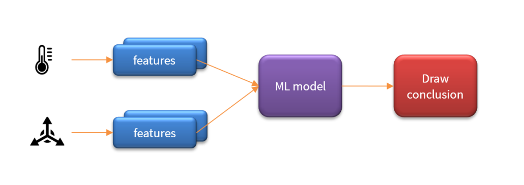
Combining the strengths of both DSP algorithms and AI/ML models leads to more robust and efficient sensor data processing systems. DSP techniques can preprocess and enhance the data, making it cleaner and more relevant for AI models to analyse. Arm Cortex processors play a pivotal role in this augmentation. Renowned for their efficiency and performance, they are widely used in AIoT (Artificial Intelligence of Things) solutions, enabling the simultaneous execution of DSP algorithms and AI/ML models directly on edge devices. This combination allows for intelligent data processing that is both rapid and power-efficient, meeting the demands of modern technology applications.
The Necessity of DSP Algorithms
DSP algorithms are essential for transforming raw sensor data into meaningful information. Sensors often collect data that is noisy or distorted, making direct interpretation challenging. DSP algorithms tackle these issues by performing noise reduction, signal enhancement, and feature extraction.
For example, the FFT converts time-domain signals into frequency-domain representations, revealing patterns crucial for applications like vibration analysis and audio. Digital filters such as lowpass, bandpass and high-pass eliminate unwanted frequency regions, isolating signals of interest and improving data quality.
Without DSP techniques, valuable insights within sensor data might remain hidden. DSP algorithms lay the groundwork by refining the data, ensuring that both traditional analysis methods and AI/ML models receive high-quality inputs. They provide reliable results based on established mathematical principles and human reasoning, which is essential in critical applications like medical devices, aerospace, and industrial automation where precision and repeatability are paramount.
As such, it’s important to realise that preprocessing of sensor data with DSP algorithms is an essential step, since AI/ML models rely heavily on the quality of input data for accurate predictions.
Moreover, DSP algorithms are efficient and can operate in real-time on devices with limited resources, such as Arm Cortex processors, making them ideal for edge computing where real-time processing is needed.
State-of-the art AIoT microcontrollers
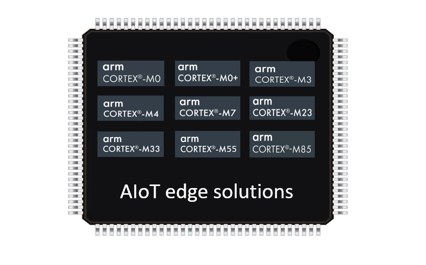
The Arm Cortex-M52, M55 and M85 are targeted for AIoT applications on microcontrollers. These processors use Arm’s powerful Armv8.1-M architecture that implement their M-Profile Vector Extension (MVE) technology (nicknamed Helium) allowing for 128bit vector mathematical operations (such as dot product operations) needed for ML and some DSP algorithms.
However, as only a few IC vendors (Alif, Ambiq, Samsung, Renesas, HiMax, Bestechnic, Qualcomm) have currently released or are planning to release any devices, Helium processors remain a gem for the near distant future.
The Necessity of AI/ML Models
While DSP algorithms are powerful, they are generally designed to address specific problems and may not scale well with the increasing complexity and volume of sensor data. AI/ML models come into play by offering the ability to learn from data, identify complex patterns, and make predictions without explicit programming for each task. They are particularly useful when:
Patterns are too complex for manual feature extraction: In cases like image and speech recognition, where the features of interest are not easily extracted using traditional DSP methods.
Data is high-dimensional or unstructured: AI/ML models can handle large datasets with numerous variables, finding relationships that may not be apparent using scientific reasoning.
Adaptive learning is required: ML models can be improved over time with more training data as it becomes available.
However, it is important to realise that AI/ML models lack common sense and are heavily reliant on the data they are trained on. As such, they may misinterpret or overlook important features if the input data is noisy or lacks proper pre-processing.
Augmenting DSP and AI/ML: a complementary approach
To maximize the benefits of sensor data processing, a hybrid approach that combines DSP algorithms with AI/ML models is often the most effective. Here’s how they complement each other:
Pre-processing with DSP:
Noise Reduction: Digital filters (e.g. lowpass) can be used to clean up the signal before it reaches the ML model.
Feature Extraction: Algorithms like FFT or DWT can extract meaningful features that reduce the dimensionality of the data and highlight important patterns.
AI/ML for Pattern Recognition:
Classification and Regression: ML models can take the features extracted by DSP algorithms and perform tasks like anomaly detection, predictive maintenance, and classification.
Adaptive Learning: ML models can adapt to new data trends over time, improving their accuracy and usefulness.
Feedback Mechanisms:
Model Refinement: The outputs from AI/ML models can inform adjustments in DSP algorithms, creating a feedback loop that enhances overall system performance.
Example Application: Vibration analysis in Industrial equipment
DSP Stage:
FFT Analysis: Converts vibration signals (usually captured from an accelerometer) from the time to frequency domain to identify characteristic frequencies associated with specific mechanical faults.
Feature Extraction: Extracts features like peak frequencies, amplitudes, and harmonics. These amplitude features can be further scaled (using properties of the FFT) to extract velocity or displacement estimates from the original acceleration data.
AI/ML Stage:
Fault Classification: An ML model trained on labelled data predicts the type of fault (e.g., imbalance, misalignment, bearing wear) based on the extracted features.
Predictive Maintenance Scheduling: Regression models estimate the remaining useful life of equipment, allowing for proactive maintenance.
Benefits of augmentation:
Improved Accuracy: Pre-processing with DSP algorithms enhances the quality of data fed into AI/ML models.
Efficiency: Reduces computational load by focusing on relevant features, which is especially important for edge devices with limited resources.
Reliability: Combining deterministic DSP outputs with probabilistic AI/ML predictions leads to more robust systems.
Detecting motor faults via harmonic fingerprint analysis
Key takeaways
The fusion of DSP algorithms and AI/ML models represents a powerful paradigm for sensor data processing in modern technology. DSP algorithms provide the necessary tools for signal enhancement and feature extraction, ensuring that the data is in the best possible form for analysis. Despite lacking any common sense (see here for a previous article), AI/ML models certainly excel at finding complex patterns and making predictions based on the processed data, making them attractive for many modern AIoT applications.
Arm Cortex processors play a pivotal role in this integration, offering the computational capabilities required to run both DSP algorithms and AI/ML models efficiently on the same platform. This synergy enables the development of advanced AIoT solutions that are capable of processing sensor data intelligently at the edge, leading to faster decisions and reduced latency. This is further strengthend with Arm’s TrustZone extension, that provides developers with a hardware data security model, offering a high level of security against hacking, stealing of encryption keys and counterfeiting.
As the volume and complexity of sensor data continue to grow, leveraging the strengths of both DSP and AI/ML will be essential for advancing technology across industries. By adopting a complementary approach and utilising decent computational platforms such as Arm’s Cortex family of processors, we can build more effective, efficient, and intelligent systems that meet the demands of the future.
Sanjeev is a RTEI (Real-Time Edge Intelligence) visionary and expert in signals and systems with a track record of successfully developing over 26 commercial products. He is a Distinguished Arm Ambassador and advises top international blue chip companies on their AIoT/RTEI solutions and strategies for I5.0, telemedicine, smart healthcare, smart grids and smart buildings.
https://www.advsolned.com/wp-content/uploads/2024/11/futuristic_sensors-scaled-e1732806588596.jpg4411029Dr. Sanjeev Sarpalhttps://www.advsolned.com/wp-content/uploads/2021/07/asn_logo_red_met_tekst_helder-e1755353934770.pngDr. Sanjeev Sarpal2024-11-28 16:03:252024-12-02 13:57:40Maximizing IoT sensor performance: Getting the most out of your sensor with DSP and AI
In modern computing, there are key concepts that define how machines process information and solve problems: Large Language Models (LLMs), algorithms, and computer programs. Each play a unique role in how tasks are performed and how intelligent systems operate.
LLMs, such as Chat-GPT, are advanced artificial intelligence models trained on massive amounts of text data to understand and generate human-like language responses. They excel at language-based tasks but rely on patterns from data rather having true intelligence based on human reasoning.
Algorithms, on the other hand, are step-by-step instructions (typically following a mathematical recipe), designed to solve specific problems or perform defined tasks. The rules or mathematical recipes that the algorithm follows have been designed by humans using reasoning and strict logic. As such, the output of the algorithm is deterministic, and can be recreate and explained by anybody following the method’s mathematical recipe or set of rules using the same input data.
Computer programs are the broader collection of code that encompasses both algorithms and models like LLMs, orchestrating various tasks by following sets of instructions. While algorithms are the building blocks for problem-solving, LLMs are specialized tools for tasks involving natural language, and programs bring these elements together to create functional software.
Understanding the differences between these three components helps clarify the architecture of modern computational systems. In this article, we discuss the differences between these terms and technologies, and provide hints and tips and a few practical examples for developers working on AIoT applications.
Programs and Algorithms: a Basic Example
A program consists of a set of instructions, often built upon one or more algorithms, to perform specific tasks based on a given input. An algorithm is a step-by-step procedure or formula for solving a problem, while a program is the implementation of that algorithm in a specific programming language.
For instance, consider a simple sorting algorithm like Bubble Sort, which can be implemented in a program:
The algorithm defines how to repeatedly compare and swap adjacent elements in a list until the list is sorted.
The program written in a language like Python or C++ implements this algorithm to sort any given list of numbers.
The key point is that a traditional program does not learn from the input or adapt its behaviour. It just follows the instructions of the algorithm every time based on the specific problem it is designed to solve.
LLMs: A Learning-Based Approach
In contrast, a Large Language Model (LLM) does not rely on predefined algorithms for specific tasks. Instead, it is trained on vast amounts of data and uses this training to predict responses based on learned patterns. For example:
If you ask an LLM to generate a recipe for pizza, it predicts the next word or sentence based on patterns it has seen in training data.
The LLM does not follow a fixed algorithm for generating recipes, but instead uses its learned understanding to predict the best response.
Unlike traditional programs, LLMs do not rely on strict rules or algorithms. They are probabilistic models that learn from a wide range of data, and their output is based on prediction rather than direct instruction.
Key Differences Between Programs and LLMs
Algorithm vs Learning: A traditional program follows strict instructions based on algorithms. LLMs, on the other hand, learn from data and use this learning to generate responses.
Fixed Output vs Prediction: In a program, the output is fixed for a given input based on the algorithm. An LLM predicts responses based on patterns, so the output can vary even with similar inputs.
No Adaptation vs Adaptation: Programs do not adapt or change their behavior unless reprogrammed. LLMs are capable of generating responses based on what they have learned, adapting to new inputs within the scope of their training.
Misconceptions about Algorithms and DLN/ML Models
Many people frequently refer to an ML model as an algorithm. This is incorrect, although the two terms are very closely related. In this section we discriminate between the two, and provide some practical examples.
Is it correct to distinguish between an ‘algorithm’ and a Deep Learning Network / ML model, as these terms are often used interchangeably but have distinct meanings?
An algorithm is a step-by-step procedure or set of rules for solving a problem, while a machine learning (ML) model is the output generated after an algorithm is applied to data during the training process. Essentially, an ML model is the learned representation or a mathematical construct based on an algorithm that can make predictions or decisions on new data.
For example, when training a neural network (which uses an algorithm like backpropagation), the result is an ML model that can classify images or recognize patterns. The algorithm guides the learning process, but the model is what performs the task after training.
What is an Algorithm?
As mentioned earlier, an algorithm is a set of rules or a mathematical recipe used to perform a specific task or to solve a problem. In ML, an algorithm is the method used to train an ML model. Examples include linear regression, decision trees, k-nearest neighbors and gradient descent.
Algorithms are very well established in the IoT sensor world for a variety of tasks, such as instrumentation and measurement, cleaning sensor data, AR (augmented reality), predictive maintenance with MEMS sensors and navigation (drones, cars and robotics). The latter makes heavy use of Kalman filtering and sensor fusion, which has been used with great success for decades.
As a simple example of an algorithm, consider the task of calculating the mean or average of set of numbers in the following dataset, \(z=[3,2,1,4,6]\). The mean can be calculated using the following mathematical recipe,
Note that this result is deterministic, in the sense that it can be recreated and more importantly explained by anybody following the function’s mathematical recipe using the same input data. This is very different to a ML model that would also reach the same result for the same input dataset, but as discussed in the next section, explaining how the model reached the result remains an enigma.
What is a DLN/ML Model?
An ML model is the resulting output or predicted result after training an algorithm on a various datasets. It typically uses various feature extraction algorithms (e.g. mean, standard deviation and correlation) during the training period in order to extract features of interest for the ML model. The resulting model represents the learned patterns, parameters, or rules that can be used to make predictions on new data.
A key point to realise here, is that unlike algorithms based on predefined rules and mathematical concepts, how the ML model reaches its result remains an enigma, and is the primary reason why they shouldn’t be allowed to operate without any scrutiny on critical processes. As such, AI systems are energy constrained Boltzmann machine models, as the model is trained on data.
In many AIoT applications, Kalman based sensor fusion is typically used for feeding the ML model with high quality features of the underlying process, thus significantly improving the accuracy of the AI system.
How Algorithms and DLN/ML Models Interact
A model provides the capability to make decisions based on input data. It can recognize patterns, make predictions, and adapt to new information. Essentially, a model simulates cognitive functions that are typically associated with human thinking, such as dealing with ambiguity and uncertainty, but as discussed in a previous article, AI does not have any common sense, as it has no understanding of the underlying data or process that it is modelling.
On the other hand, an algorithm is a set of defined instructions or a mathematical recipe. It is a rules based step-by-step procedure used for calculations, data processing, and automated reasoning tasks. Algorithms are the backbone of software and can solve a wide range of problems by following their defined logic.
However, not all functions are computable. This means that there are certain problems for which no algorithm can be formulated to provide a solution. These are referred to as non-computable functions. In such cases, even the most advanced algorithms cannot determine an outcome, highlighting a fundamental limitation in computational theory.
Human Intelligence and Digital Intelligence
In the field of computation, it is essential to differentiate between traditional algorithms and machine learning models. An algorithm is a direct output of human intelligence, crafted through logical reasoning and problem-solving techniques. It represents a set of predefined instructions designed to solve specific problems. The human mind formulates these steps to ensure a consistent and accurate outcome.
In contrast, a trained machine learning (ML) model is the product of digital intelligence. While algorithms underpin the model’s structure, the true power of an ML model arises through its capacity to learn and adapt from new training data. This process involves iteratively adjusting parameters to optimize performance in tasks like prediction, classification, or decision-making. In this sense, the model evolves beyond its initial algorithmic foundation, generating insights and results that may not be directly encoded by human logic.
“An algorithm is a direct manifestation of human intelligence, designed through logic, reasoning, and problem-solving techniques. On the other hand, a trained machine learning model represents the outcome of digital intelligence, which evolves through the iterative processing of data.”
The convergence of these two forms of intelligence—human and digital—marks a significant shift in computational systems. Algorithms, though foundational, are static and require manual updates. Machine learning models, by contrast, learn from experience, dynamically evolving with each new piece of training data. This shift positions ML models as more flexible and adaptive tools for solving complex problems where human-defined rules may fall short.
The distinction between human-driven algorithms and data-driven machine learning models emphasizes the growing role of adaptive systems in areas such as autonomous driving, personalized medicine, and financial forecasting. As machine learning continues to evolve, the boundaries between explicit programming and emergent behavior will continue to blur, paving the way for systems capable of independent learning and decision-making.
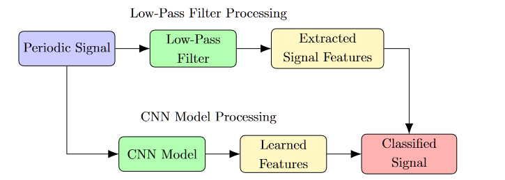
Low-Pass Filter and CNN for Classifying Periodic Signals
Both a Low-Pass Filter (LPF) and a Convolutional Neural Network (CNN) can be employed to handle periodic signals, but their approaches and purposes differ fundamentally.
Low-Pass Filter (LPF)
A Low-Pass Filter is an algorithm designed to attenuate the high-frequency components of a signal while allowing the low-frequency components to pass. Its primary use is to filter or clean a signal rather than classify it. Applications of the LPF in AIoT, include removing glitches from sensor data or even cleaning up noise on a measured periodic signal prior to feature extraction and subsequent ML classification, leading to higher accuracy.
A practical IIR (infinite impulse response) digital filter used in both AIoT and IoT may be defined in terms of a finite number of poles \(p\) and zeros \(q\), as defined by the linear constant coefficient difference equation,
where, \(a_k\) and \(b_k\) are the filter’s denominator and numerator polynomial coefficients, who’s roots are equal to the filter’s poles and zeros respectively. LPF filter can used for all types of signals, not just periodic signals. However, for this article we limit the discussion to periodic signals.
Limitations for Classification
While an LPF can enhance a periodic signal by reducing high-frequency noise, it does not classify the signal. It merely transforms the input based on fixed mathematical operations, with no ability to learn from data or adapt its behaviour.
Convolutional Neural Network (CNN)
A Convolutional Neural Network (CNN) is a machine learning model designed to recognize patterns in data by learning from training examples. It can be trained to classify periodic signals by learning distinctive features in the signal’s structure.
Operation
The CNN applies a series of convolution operations:
where \(I\) is the input signal, \(K\)is the kernel, and \(S(i,j)\) is the resulting feature map.
Classification
Unlike the LPF, the CNN is capable of learning to classify different periodic signals through training. The learned filters allow the network to distinguish between signals based on the periodic features it identifies.
Extraction vs Learned feature
Low-Pass Filter: Performs a deterministic operation that modifies the signal but cannot classify it.
CNN: Learns from data and can classify periodic signals by recognizing their features.
In conclusion, while a Low-Pass Filter may assist in signal preprocessing, a CNN is required for the task of classifying signals.
Adaptive Low-Pass Filters
An adaptive low-pass filter (LPF), such as those based on the Least Mean Squares (LMS) algorithm, introduces several key features and benefits compared to a traditional, static LPF:
Dynamic Adaptability: Adaptive LPFs adjust their characteristics in response to variations in the input signal, allowing for real-time filtering of noise or unwanted frequencies, especially in non-stationary signals.
Error Minimization: These filters utilize a feedback mechanism to minimize the difference (error) between the desired output and the actual output. The filter coefficients are continuously updated based on this error, enhancing the filter’s adaptability to changing signal conditions.
Improved Performance in Noisy Environments: Adaptive LPFs effectively reduce noise by optimizing signal quality, which is particularly valuable in applications like audio processing, telecommunications, and biomedical signal processing where signal characteristics can fluctuate.
Applications in Real-Time Systems: The adaptability of these filters makes them suitable for real-time systems, such as echo cancellation in telecommunication, where the noise characteristics may vary dynamically, ensuring consistent performance over time.
Computational Complexity: While adaptive filters provide significant advantages, they also come with increased computational complexity due to the need for constant updates to the filter coefficients, which can be a concern in systems with limited processing capabilities.
In summary, using an adaptive LPF enhances the filter’s ability to handle varying signal conditions effectively, making it particularly valuable in applications requiring real-time signal processing, thus improving overall performance and robustness against noise and interference.
Adaptive low-pass filter (LPF) differs significantly from a traditional LPF in terms of feature extraction and learning capabilities.
Feature Extraction vs. Feature Learning
Traditional LPF: This filter focuses on extracting specific frequency components from a signal by applying fixed coefficients determined by the filter design, which remain constant during operation. As a result, it extracts features based on pre-defined criteria.
Adaptive LPF: Utilizes algorithms like the Least Mean Squares (LMS) to adjust its filter coefficients in real-time based on the input signal characteristics. This enables the adaptive LPF to extract features that dynamically correspond to changing signal conditions, but it does not learn features in the same manner as a neural network.
Comparison with CNNs
Convolutional Neural Networks (CNNs): CNNs are designed to learn features from data through multiple layers, allowing them to automatically extract high-level features from raw inputs. Unlike traditional LPFs, CNNs perform feature learning, adapting to the input data through training on labeled datasets.
While adaptive LPFs adjust their response based on signal changes, they do not perform feature learning like CNNs. They can optimize their filter characteristics based on feedback but lack the hierarchical feature learning approach present in CNNs.
Adaptive LPFs can extract features based on the immediate conditions of the signal; however, they do not ‘learn’ features in the same way that CNNs do. Instead, adaptive LPFs optimize the extraction process in real-time, making them effective in environments where signal characteristics vary.
Comparison of Adaptive Low-Pass Filters and Convolutional Neural Networks
Adaptive low-pass filters (LPFs), such as those using the Least Mean Squares (LMS) algorithm, exhibit several similarities with convolutional neural networks (CNNs) regarding their operational principles and learning mechanisms.
Adaptive Coefficients: Adaptive LPFs modify their coefficients based on the input signal, similar to how CNNs adjust their weights during training to minimize loss on a dataset.
Supervised Learning: Both systems can be trained using labeled data to optimize performance. Adaptive filters adjust based on real-time feedback while CNNs learn complex patterns through multiple iterations.
Feature Extraction: Adaptive LPFs extract relevant features dynamically, while CNNs automatically learn to identify hierarchical features through their architecture.
Learning Methodology: Adaptive LPFs adjust their parameters based on incoming data but do not learn complex representations as CNNs do. CNNs can learn multiple levels of abstraction through backpropagation.
Structure and Complexity: CNNs consist of multiple layers, allowing them to learn intricate patterns, whereas adaptive LPFs typically operate with a single, simpler structure focused on modifying coefficients.
Items 1,2 and 3 are similar, but item 4 and 5 are different.
While adaptive LPFs and CNNs share similarities in their adaptive behaviors and feature extraction capabilities, they fundamentally differ in methodologies and complexities. Adaptive LPFs do not fully replicate the intricate learning capabilities of CNNs, though both aim to improve task performance through adaptation.
Comparison of Adaptive LPFs and CNNs
Order of the Filter: The order of an adaptive low-pass filter (LPF) determines its ability to capture and process complex signal characteristics. A higher-order filter can approximate a more complex frequency response, allowing it to better handle diverse signal patterns, similar to how a deeper convolutional neural network (CNN) can learn more complex representations.
Learning Capabilities: While both CNNs and adaptive LPFs adjust their parameters based on input, CNNs inherently possess a more advanced learning capability through multiple layers, each designed to extract different levels of abstraction from the data. This allows CNNs to learn hierarchical feature representations effectively. In contrast, increasing the order of an adaptive LPF can enhance its feature extraction capabilities, but it still lacks the sophisticated learning mechanisms that CNNs implement, such as backpropagation and convolutional operations.
Complex Features: CNNs excel in extracting spatial hierarchies in data (e.g., images) by applying filters across multiple layers, progressively identifying edges, shapes, and more abstract features. Adaptive LPFs, when designed with a higher order, can capture complex signal behaviours, but their ability to generalize or learn from large datasets is limited compared to CNNs.
While increasing the order of an adaptive LPF can enhance its performance in signal processing, it does not equate to the deep learning capabilities of CNNs. CNNs utilize their layered architecture to learn complex features in a more robust and generalized manner, making them more suitable for tasks like image recognition and classification.
Parameter Estimation
Parameter estimation plays a crucial role in both traditional algorithmic processes and machine learning. It involves determining the best parameters for a given model based on observed data.
Algorithmic Parameter Estimation
In traditional algorithmic contexts, parameter estimation involves using specific algorithms to find optimal parameters for mathematical models. Key methods include:
Least Squares Estimation (LSE)
This method minimizes the sum of the squared differences between observed and predicted values. The parameter estimation is given by:
where \(\hat{\theta}\) denotes the estimated parameters. this concept is is central to Kalman filtering, whereby a state-space model of the process to be modelled uses the state estimates (i.e. the parameters of interest) to perform the prediction. The Kalman update equations attempt to minimise the error between the model output and the observed data in a least squares sense on a sample-by-sample basis.
Maximum Likelihood Estimation (MLE)
MLE estimates parameters by maximizing the likelihood function, which reflects the probability of the observed data under the model parameters:
where \(p(\theta | \text{data})\) is the posterior distribution.
In both traditional algorithms and machine learning contexts, the aim is to find the optimal parameters that best fit the model to the observed data.
Key Takeaways
Many people frequently refer to an ML model as an algorithm. This is incorrect, although the two terms are very closely related. An algorithm is a direct output of human intelligence, crafted through logical reasoning and problem-solving techniques. It represents a set of predefined instructions or a mathematical recipe designed to solve specific problems. The human mind formulates these steps to ensure a consistent and accurate outcome. In contrast, a trained machine learning (ML) model is the product of digital intelligence that uses algorithms and datasets to construct an ML model.
A key takeaway is that algorithms are based on predefined rules and mathematical concepts, whereas AI systems are energy constrained Boltzmann machine models, as the model is trained on data. As such, how an ML model reaches its result remains an enigma, and is the primary reason why they shouldn’t be allowed to operate without any scrutiny on critical processes.
Sanjeev is a RTEI (Real-Time Edge Intelligence) visionary and expert in signals and systems with a track record of successfully developing over 26 commercial products. He is a Distinguished Arm Ambassador and advises top international blue chip companies on their AIoT/RTEI solutions and strategies for I5.0, telemedicine, smart healthcare, smart grids and smart buildings.
Jayakumar is an Arm ambassador and seasoned expert in semiconductor technology and AIoT. He advices companies such as Mistral Solutions, SunPlus Software, and Apollo Tyres at the strategic level on their AIoT solutions. He successfully founded Epigon Media Technologies, which focuses on Research and Development for the global market, and is also the co-author of the book "Deep Learning Networks: Design, Development, and Deployment."
https://www.advsolned.com/wp-content/uploads/2024/10/robot_reading-scaled-e1729851827745.jpg7201080Dr. Sanjeev Sarpalhttps://www.advsolned.com/wp-content/uploads/2021/07/asn_logo_red_met_tekst_helder-e1755353934770.pngDr. Sanjeev Sarpal2024-10-25 12:27:242024-10-25 14:30:58An AI/ML model is not an algorithm
In the rapidly evolving landscape of digital transformation, organizations are increasingly leveraging Real-Time Edge Intelligence (RTEI) solutions to enhance operational efficiency and decision-making capabilities. RTEI refers to the deployment of advanced data processing and analytics at the edge of the network (i.e. closer to where data is generated) rather than relying solely on centralized cloud infrastructure. This approach successfully addresses the challenges posed by traditional data processing methods and offers significant benefits across multiple sectors, particularly when building solutions with Arm processor technology.
Key concepts of Real-Time Edge Intelligence
Improved Response Times: RTEI enables immediate data processing and analysis, resulting in faster decision-making. For industries like healthcare, manufacturing, and transportation, this can mean the difference between success and failure in critical situations. Arm processors allow for high-performance computing in compact form factors, making them ideal for real-time applications.
DSP/ML at the Edge: Arm’s extensive ecosystem of partner solutions and in-built algorithmic accelerator technology makes deploying DSP algorithms and ML models on the edge very easy. This enables RTEI solutions to provide real-time insights and predictions of the process that they’re monitoring, empowering organizations to automate processes and respond dynamically to changing conditions.
Data cleaning and feature extraction: Arm-based devices can clean noisy sensor data and extract features interest at the edge, sending only relevant data to the cloud. This minimizes bandwidth usage and optimizes network performance, ensuring that only critical data is transmitted. Arm’s low-power architecture is ideal for this task, allowing devices to perform complex computations in battery-powered applications.
Cost Efficiency: By reducing the amount of data sent to the cloud, organizations can lower bandwidth costs and cloud storage expenses. The efficient processing capabilities of Arm processors allow for more effective resource use, leading to operational cost savings. Their energy efficiency further contributes to reduced operational costs in large-scale deployments.
Increased Reliability: RTEI solutions can operate independently of cloud connectivity, ensuring that essential mission-critical applications continue to function even during a network outage. The robustness of Arm technology in various environmental conditions enhances system reliability and operational resilience, particularly in remote locations, typically encountered in many IoT applications.
Scalability: Arm-based solutions can be easily scaled to accommodate growing data volumes and an increasing number of connected devices. The modularity of Arm architecture supports the development of a diverse ecosystem of devices, making it easier for organizations to adapt to changing business needs.
Enhanced security and privacy with Arm TrustZone
Security is a critical concern for edge devices, particularly those handling sensitive data. Arm TrustZone (Cortex-M33, Cortex-M52 and Cortex-A) implements a security paradigm that discriminates between the running and access of untrusted applications running in a Rich Execution Environment (REE) and trusted applications (TAs) running in a secure Trusted Execution Environment (TEE). The basic idea behind a TEE is that all TAs and associated data are secure as they are completely isolated from the REE and its applications. As such, this security model provides a high level of security against hacking, stealing of encryption keys, and counterfeiting, and as such provides an elegant way of protecting sensitive client information.
DSP support for Algorithms
DSP is critical for many RTEI applications, including audio and video processing, sensor signal processing and data analysis. Arm’s broad range of processors offer extensive DSP capabilities, allowing for the implementation of complex algorithms in floating-point. The Cortex-M family dominates the low-power micro-controller market as described below, whereas the more powerful Application or Cortex-A processors target mini-computers, such as the Raspberry Pi and smartphones etc. The Cortex-R family targets real-time safety-critical applications, such as automotive and radar.
All three types of processors offer algorithmic support, but the Cortex-M family is particularly interesting, as it adds DSP functionality to low-power microcontroller devices making it highly desirable for the IoT market, as we now discuss in the following section.
Cortex-M processors
Although a few processor technologies exist for microcontrollers (e.g. RISC-V, Xtensa, MIPS), over 90% of the microcontrollers used in the smart product market are powered by so-called Arm Cortex-M processors that offer a combination of high algorithmic performance, low-power and security. The Arm Cortex-M4 is a very popular choice with several silicon vendors (including ST, TI, NXP, ADI, Nordic, Microchip, Renesas), as it offers DSP (digital signal processing) functionality traditionally found in more expensive devices and is low-power.
Acceleration of DSP calculations
The Armv7E-M architecture supports a DSP extension that implements an SIMD (single instruction, multiple data) architecture extension that can significantly improve the performance of an algorithm. The basic idea behind SIMD involves parallel execution of an instruction (e.g. Add, Subtract, Multiply, Divide, Abs etc) on multiple data elements via the use of 64 or 128-bit registers. These DSP extension intrinsics (SIMD optimised instruction) support a variety of data types, such as integers, floating and fixed-point.
The high efficiency of the Arm compiler allows for the automatic dissemination of your C code in order to break it up into SIMD intrinsics, so explicit definition of any DSP extension intrinsics in your code is usually unnecessary. The net result for your application is much faster code, leading to better power consumption and for wearables, better battery life.
What algorithmic operations would use this?
The following examples give an idea of operations that can be significantly speeded up with SIMD intrinsics:
vadd can be used to expedite the calculation of a dataset’s mean. Typical applications include average temperature/humidity readings over a week, or even removing the DC offset from a dataset.
vsub can be used to expedite numerical differentiation in peak finding for a sinewave tracking application.
vabs can be used for expediting the calculation of an envelope of a fullwave rectified signal in EMG biomedical and smartgrid applications.
vmul can be used for windowing a frame of data prior to FFT analysis. This is also useful in audio applications using the overlap-and-add method.
The hardware floating point unit is very good for expediting MAC (multiply and accumulate) operations used in digital filtering, requiring just three cycles to complete. Other DSP operations such as add, subtract, multiply and divide require just one cycle to complete.
Key takeaways
As organizations continue to embrace digital transformation, Real-Time Edge Intelligence (RTEI) solutions, particularly when integrated with Arm processor technology, stand out as key enablers of innovation and efficiency. By harnessing the power of edge computing and the performance advantages of Arm’s Cortex-A and Cortex-M architectures, the security benefits of Arm TrustZone, and the DSP capabilities for advanced algorithms, businesses can achieve rapid decision-making, enhance security, and optimize operational costs. The future of data processing lies at the edge, and those who adopt RTEI solutions powered by Arm technology will be well-positioned to thrive in an increasingly competitive landscape.
Sanjeev is a RTEI (Real-Time Edge Intelligence) visionary and expert in signals and systems with a track record of successfully developing over 26 commercial products. He is a Distinguished Arm Ambassador and advises top international blue chip companies on their AIoT/RTEI solutions and strategies for I5.0, telemedicine, smart healthcare, smart grids and smart buildings.
Over the last few years, there has been tremendous interest in the possibility of replacing humans at the workplace with AI. One obvious advantage is AI’s ability to process massive amounts of data and perform tasks such as repetitive tasks (such as data entry) much more efficiently than humans, leading to higher productivity and reduced operational costs. AI can also work continuously without fatigue, ensuring 24/7 customer service. However, can AI truly think and rationalise like a human?
Challenges in understanding of the real-world
Our experience with AI systems suggests categorically that AI’s current limitation is that it does not have any common sense, as there is no reasoning component in the current generation AI model-based inference. As such, current AI does not truly understand the world the way humans do. AI models are trained on large datasets, which are essentially collections of text, images, sensor data etc, and generates responses based on statistical correlations in data. While they can learn patterns and extract important features from this data, they don’t inherently understand the meaning of this data. Understanding is a fundamental component of human intelligence and commonsense, allowing us to take actions and draw conclusions that may seem logical to some, but irrational to people with other experiences in life. In short, we can conclude that commonsense is built up from real-world experiences, social interactions, emotions and context, which is something that AI currently lacks.
The aforementioned acknowledges that current AI models lack commonsense due to the absence of reasoning components. Also, there is the potential for AI models to converge on solutions that may not adhere to Bayesian learning principles, which is an important consideration. We’ll now look at this aspect in depth with a few examples, but we’ll start off with examples of where having no common sense can be turned to an advantage.
Transparency and fake news
Having no common sense and no real understanding of the data can also be turned into an advantage. Consider the example of an AI sorting through CVs (resumes) of suitable candidates for a job. The model can be limited to just focus on the work experience and education, and ignore the name, gender and nationality, making the process much more transparent. Humans will generally try and form a picture in their heads about the candidate and may then appraise the CV with prejudice rather than merit.
Perhaps one of the best examples of AI has been in the media. Whereby a model can be fed with a certain narrative (e.g. anti-abortion or pro-war) and then instructed to produce a new article, filling in the details with arbitrary photos and facts taken from other media sources, and older publications. Many of the articles are not verified by an editorial team before publication, resulting in unconfirmed stories making it to the news websites. This is not just limited to news, reviewers of several scientific publications have also reported fake articles sent for review – some of which have been published, which is an area of concern for the scientific community.
Is it a Dog or a Cat?
Consider an AI model trained to classify images of animals. The model can accurately classify images of cats and dogs when presented with typical images of these animals. However, when presented with an unusual image, the model might fail to classify it correctly due to the lack of reasoning and common sense.
For instance, if the AI model is given an image of a cat wearing a dog costume, it might classify the image as a dog because it lacks the reasoning component to understand that the core features of a cat are still present despite the costume. A human, using common sense, would easily identify the animal as a cat in a dog’s costume.
In this example, the AI model converges on a solution that classifies the image as a dog, which may disobey Bayesian learning principles that consider the prior probability of encountering a cat versus a dog in such a context.
This limitation highlights the importance of integrating reasoning components into AI models to enhance their common sense and improve their ability to handle unusual or unexpected situations effectively.
Bayesian learning enhances deep learning networks by providing uncertainty quantification, preventing overfitting, facilitating model comparison, enabling data-efficient learning, and improving interpretability. This makes Bayesian approaches highly valuable in critical applications where reliability, robustness, and transparency are paramount. More information can be found in the following video.
Data vs Science for IoT T&M applications
Many IoT test and measurement (T&M) and calibration methods use sinewaves to check compliance of the DUT (device under test) by measuring the sinewave’s amplitude, some examples include:
Measuring material fatigue/strain with a loadcell – in vehicle and bridge/building applications measuring material fatigue and strain is essential for safety. An AC sinusoidal excitation overcomes the difficulty of dealing with instrumentation electronics DC offsets.
Calibrating CT (current transformers) sensors channels – a sinusoid of known amplitude is applied to channel input and the output amplitude is measured.
Measuring gas concentration in infra-red gas sensors – the resulting sinusoid’s amplitude is used to provide an estimate of gas concentration.
Measuring harmonic amplitudes in power quality smart grids applications – in 50/60Hz power systems, certain harmonic amplitudes are of interest.
ECG biomedical compliance testing (IEC60601-2-47) – channel compliance with IEC regulations needed for FDA testing typically uses a set of sinewaves at known amplitudes, to ensure that the channel’s signal chain amplitude error is within specification.
The latter example is particularly interesting, as the basic idea is to measure the amplitude differences in the DUT’s signal chain for a set of sinewaves at 0.67, 1, 2, 10, 20 and 40Hz with respect to a 5Hz reference sinewave. Where, it is assumed the amplitude of all input sinewaves remains constant, and that the relative amplitude error must be within ±3dB for the signal chain to be classed as IEC compliant.
There are a number of signal processing methods that can be employed to perform the estimation, such as the FFT, AM modulation, Hilbert transform and full-wave rectification. All of these methods require extra filtering operations and the FFT for examples, requires low frequency trend removal (usually a DC offset), and windowing so there a number of factors to take into consideration, which complicates the challenge. The FFT is perhaps one of the most widely used methods but is limited by its frequency resolution, which leads to a bias on the amplitude estimate if it’s not centred at a multiple of the ideal frequency bin resolution (\(F_s/N\)).
As most IoT devices use a low-cost oscillator, the sampling rate error can be as high as ±3%, leading to a significant bias in the amplitude estimation using the FFT method. Therefore, an important first step for establishing an estimate of the sinewave’s amplitude is to estimate the exact sampling frequency of the DUT.
Another simpler method that we’ve seen on some IoT devices, is to use high time-resolution timestamps from a higher accuracy crystal oscillator, but for lower-cost IoT devices this may not be available, so it’s better to have a strategy that extracts the exact sampling rate from the dataset.
Sampling rate estimation using AI
Sampling rate estimation can be achieved using AI, whereby datasets of the known input test sinewaves are collected for subsets of the ideal sampling rate. For many IoT ECG devices, 200Hz is typically used. Therefore, assuming an ideal sampling rate of 200Hz, we can generate test sinewave data sampled at 199.5Hz, 199.6Hz…..200.4Hz, 200.5Hz etc. This collection of sinewave data can then be fed into an ML classifier for estimation of the true sampling rate. Assuming that the training dataset is large enough to cover all required scenarios, this method will work.
However, it should be noted that this approach doesn’t have any commonsense, since it’s purely based on data and has no understanding of the physical process that it’s modelling. This becomes apparent if the sampling error is, say 199.54Hz. As the model doesn’t have any data for this scenario and doesn’t have any commonsense and as such can’t improvise, it must choose between 199.5Hz and 199.6Hz which will lead to a bias in the true sampling rate estimate. Another problem appears if another sampling rate or other test frequencies are used, as these were not taken into account during the training process.
Sampling rate estimation using a UKF
An alternative approach is to model the physical process using an Unscented Kalman Filter (UKF). The UKF’s flexibility allows for a more detailed mathematical model of the process to be implemented, leading to the possibility of estimating the sinewave’s amplitude, phase, DC offset as well as the true sampling rate.
Assuming stationarity, a mathematical model of the process can be described as,
Where, \(\theta\) is initial phase offset, \(v(n)\) is the measurement noise and \(A\) (sinewave’s amplitude), \(B\) (signal’s DC offset) and \(F_s\) (sampling rate) are the parameters that we want to estimate.
This model can be broken down and the entities of interest (\(A, B\) and \(F_s\)) implemented as state variables in the Kalman update equations. Notice that although the phase of sinewave is linear, the output of the \(\sin()\) function is non-linear, which means that the relationship between the observed signal to the entity of interest (\(F_s\) in our case) is non-linear. This is the main reason for choosing the UKF, as it is well suited to handling non-linear relationships. A description of the UKF equations is beyond the scope of this article, but the reader is referred to some of the excellent textbooks on the UKF for a complete description of the algorithm.
Assuming that the test sinewave is high accuracy – a realistic assumption since a modern calibrated signal generator has frequency error in the \(\mu\)Hz region, we can use the Kalman filtering equations to estimate the true sampling rate over time. An important to point to realise is that like the AI method described above, the UKF also doesn’t have any commonsense, but has the virtue of ‘understanding’ the process that it’s modelling by virtue of the mathematical model implemented in its update equations. This means that a sinewave of any frequency and sampling rate can be applied to the UKF, and assuming that the exact sinewave frequency is also entered into the state equations, the UKF method will always work.
However, one potential weakness of the method for this application is that the Kalman filter is a statistical state estimation method, meaning that its state estimation will be optimal in a statistical sense, but not necessarily in a deterministic sense. This means that there is no guarantee that the state estimates will be correct in a deterministic (absolute) sense.
An animation of the UKF estimation for a 32.3Hz sinewave, sampled at 100Hz with a 0.1% sampling rate error (100.1Hz) is shown below, as seen the UKF correctly estimates the state-estimates of the test sinewave within 1 second.
AI in weapons technology
Recently, much emphasis has been placed on developing smart weapons using AI technology. Major weapons manufacturers from all over the world are currently experimenting with AI-based drone technology that can be used to attack enemy combatants in swarms as well deploying GPS-guided smart munitions and developing new EW (electronic warfare) jamming technology.
Many Western nations allocate substantial resources to defence spending, with significant portions of their budgets dedicated to military operations and technological advancements. However, modern conflict zones highlight the evolving challenges that defence systems face, particularly in terms of operational complexity and sustainability in international theatres of operation.
Looking further to the East, nations such as Russia and China allocate a much smaller budget to their military-industrial complex. Their approach focuses instead on utilizing AI in a more targeted manner, emphasizing established scientific and mathematical principles, such as control theory, with AI applied for classification purposes. Over recent years, as repeatly demostrated in various international conflict zones, this strategy has proven to be very effective. Technologies like hypersonic missiles and electronic warfare systems developed by Russia have managed to evade many Western air defense systems, altering the balance of power in several theatres of operation. This impressive performance challenges the notion that simply investing large sums of money into AI weapons technology guarantees superior results.
Returning to the subject at hand, all of these AI smart weapons still lack any common sense as the AI cannot reason like a human. As such, it is dangerous to allow these systems to operate autonomously and to have high expectations of their performance in a combat situation. That being said, researchers working at Russia’s AIRI research institute contend to have taken significant steps forward in developing the world’s first self-learning AI system (Headless-AD) that can adapt to new situations/tasks without any human intervention by autoregressively predicting actions using the AI’s existing learning history model as context. If successful, Headless-AD would be a great leap forward in developing sentient AI technology for all walks of life.
Human Intelligence and Digital Intelligence
In the field of computation, it is essential to differentiate between traditional algorithms and machine learning models. An algorithm is a direct output of human intelligence, crafted through logical reasoning and problem-solving techniques. It represents a set of predefined instructions designed to solve specific problems. The human mind formulates these steps to ensure a consistent and accurate outcome.
In contrast, a trained machine learning (ML) model is the product of digital intelligence. While algorithms underpin the model’s structure, the true power of an ML model arises through its capacity to learn from large scale data. This process involves adjusting parameters during the training period (not during the inference time/runtime) to optimize performance in tasks like prediction, classification, or decision-making. In this sense, the model evolves beyond its initial algorithmic foundation, generating insights and results that may not be directly encoded by human logic.
An algorithm is a direct manifestation of human intelligence, designed through logic, reasoning, and problem-solving techniques. On the other hand, a trained machine learning model represents the outcome of digital intelligence, which evolves through the iterative processing of data.
The convergence of these two forms of intelligence—human and digital—marks a significant shift in computational systems. Algorithms, though foundational, are static and require manual updates. Machine learning models, by contrast, can be improved by providing them with more training data when available. This shift positions ML models as more flexible and adaptive tools for solving complex problems where human-defined rules may fall short.
The distinction between human-driven algorithms and data-driven machine learning models emphasizes the growing role of adaptive systems in areas such as autonomous driving, personalized medicine, and financial forecasting. As machine learning continues to evolve, the boundaries between explicit programming and emergent behavior will continue to blur, paving the way for systems capable of independent learning and decision-making.
Key takeaways
There has been considerable interest in the potential of replacing human roles in the workplace with AI. However, as discussed herein, AI fundamentally lacks an understanding of the meaning behind the data it processes for classification tasks. This ‘lack of understanding’ is a core component of human intelligence and common sense, which enables individuals to make decisions and draw conclusions that may appear logical to some but irrational to others based on varying life experiences. In essence, common sense is derived from real-world experiences, social interactions, emotions, and context—attributes that AI currently lacks and is unlikely to acquire in the foreseeable future.
Nevertheless, the absence of common sense and a deep understanding of data can also be leveraged to create a more transparent process for job applicants and application reviews. Conversely, AI can be utilized to generate misleading information shaped by influential entities to support specific narratives and sway public opinion.
Sanjeev is a RTEI (Real-Time Edge Intelligence) visionary and expert in signals and systems with a track record of successfully developing over 26 commercial products. He is a Distinguished Arm Ambassador and advises top international blue chip companies on their AIoT/RTEI solutions and strategies for I5.0, telemedicine, smart healthcare, smart grids and smart buildings.
Jayakumar is an Arm ambassador and seasoned expert in semiconductor technology and AIoT. He advices companies such as Mistral Solutions, SunPlus Software, and Apollo Tyres at the strategic level on their AIoT solutions. He successfully founded Epigon Media Technologies, which focuses on Research and Development for the global market, and is also the co-author of the book "Deep Learning Networks: Design, Development, and Deployment."
https://www.advsolned.com/wp-content/uploads/2024/09/Robot_thinking.jpg19911991Dr. Sanjeev Sarpalhttps://www.advsolned.com/wp-content/uploads/2021/07/asn_logo_red_met_tekst_helder-e1755353934770.pngDr. Sanjeev Sarpal2024-09-17 15:54:062024-09-17 16:16:26From IoT to AIoT: is it true that AI doesn’t have any common sense?
AI (Artificial Intelligence) has its roots with the famous mathematician Alan Turing, who was the first known person to conduct substantial research into the field that he referred to as machine intelligence. Turing’s work was published as Artificial Intelligence and was formally categorised as an academic discipline in 1956. In the years following, work undertaken at IBM by Arthur Samuel led to the term Machine Learning, and the field was born.
In terms of definitions: AI is an umbrella term, whereas ML (Machine Learning) is a more specific subset of AI focused on producing inference using trained networks. During training, the dataset plays a key role in ML quality during inference. AI provides scope for ML and Deep Learning. In fact, Deep Learning Networks use amazing Transformer models for the current generation AI world.
AI is the overarching field focused on creating intelligent systems, whereas ML is a subset of AI that involves creating models to learn from data and make decisions.
ML is crucial for IoT because it enables efficient data analysis, predictive maintenance, smart automation, anomaly detection, and personalized user experiences, all of which are essential for maximizing the value and effectiveness of IoT deployments.
The difference between AI and ML in a nutshell
Artificial Intelligence (AI):
Definition: AI is a broad field of computer science focused on creating systems capable of performing tasks that normally require human intelligence. These tasks include reasoning, learning, problem-solving, perception, and language understanding.
Scope: Encompasses a wide range of technologies and methodologies, including machine learning, robotics, natural language processing, and more.
Example Applications: Voice assistants (e.g., Siri, Alexa), autonomous vehicles, game-playing agents (e.g., AlphaGo), and expert systems.
Machine Learning (ML):
Definition: ML is a subset of AI that involves the development of algorithms and statistical models that enable computers to learn from and make predictions or decisions based on data.
Scope: Focused specifically on creating models that can identify patterns in data and improve their performance over time without being explicitly programmed for specific tasks.
Example Applications: Spam detection, image recognition, recommendation systems (e.g., Netflix, Amazon), predictive maintenance of critical machinery and identifying medical conditions, such as heart arrhythmias and tracking vital life signs – the so called IoMT (Internet of Medical Things).
Why We Need ML for IoT
Data Analysis:
Massive Data: IoT devices generate a vast amount of data. ML is essential for analyzing this data to extract meaningful insights, detect patterns, and make informed decisions.
Real-Time Processing: ML models can process and analyze data in real-time, enabling immediate responses to changes in the environment, which is crucial for applications like autonomous vehicles and smart grids. They are also an invaluable tool for monitoring human well-being, such as tracking vital life signs, and checking motion sensor data for falls and epileptic fits in elderly and vulnerable persons.
Automation:
Smart Automation: ML enables IoT devices to automate complex tasks that require decision-making capabilities, such as adjusting climate control systems in smart buildings based on occupancy patterns.
Adaptability: ML models can adapt to changing conditions and improve their performance over time, leading to more efficient and effective automation.
Personalization:
User Experience: ML can analyze user preferences and behaviors to personalize experiences, such as recommending products, adjusting device settings, or providing personalized health insights from wearable devices.
Enhanced Interaction: Improves the interaction between users and IoT devices by making them more intuitive and responsive to individual needs.
What is AIoT exactly?
IoT nodes or edge devices use convolutional neural networks (CNN) or neural networks (NN) to perform inference on data collected locally. These devices can include cameras, microphones, or UAV-based sensors. By having the ability to perform inference locally on IoT devices, it enables intelligent communication or interaction with these devices. Other devices involved in the interaction can also be IoT devices, human users, or AIoT devices. This creates opportunities for AIoT (Artificial Intelligence of Things) rather than just IoT, as it facilitates more advanced and intelligent interactions between devices and humans.
AIoT is interaction with another AIoT. In this case, there is a need for artificial intelligence on both sides to have a meaningful interaction.
AIoT is interaction with IoT. In this case, there is a need for artificial intelligence on one side, and no AI on the other side. Thus, it is not a good and safe configuration for deployment.
AIoT is interaction with a human. In this case, there is a need for artificial intelligence on one side and a human on the other side. This is a good configuration because the volume of data from the device to the human will be less.
Human Also in the Loop is a Thing of the Past
Historically, humans have used sensor devices, now referred to as IoT edges or nodes, to perform measurements before making decisions based on a particular set of data. In this process, both humans and IoT edge devices participate. Interaction between one IoT edge and another is common, but typically within restricted applications or well-defined subsystems. With the rise of AI technologies, such as ChatGPT and Watsonx, AI-enabled IoT devices are increasingly interacting with other IoT devices that also incorporate AI. This interaction is prevalent in advanced driver-assistance systems (ADAS) with Level 5 autonomy in vehicles. In earlier terms, this concept was known as Self-Organizing Networks or Cognitive Systems.
The interaction between two AIoT systems introduces new challenges in sensor fusion. For instance, the classic Byzantine Generals Problem has evolved into the Brooks-Iyengar Algorithms, which use interval measurements instead of point measurements to address Byzantine issues. This sensor fusion problem is closely related to the collaborative filtering problem. In this context, sensors must reach a consensus on given data from a group of sensors rather than relying on a single sensor. Traditionally, M measurements with N samples per measurement produce one outcome by averaging data over intervals and across sensor measurements.
Sensor fusion involves integrating data from multiple sensors to obtain more accurate and reliable information than what is possible with individual sensors. By rethinking this problem through the lens of collaborative filtering—an approach widely used in recommendation systems—we can uncover innovative solutions. In this analogy, sensors are akin to users, measurements are comparable to ratings, and the environmental parameters being measured are analogous to items. The goal is to achieve a consensus measurement, similar to how collaborative filtering aims to predict user preferences by aggregating various inputs. Applying collaborative filtering techniques to sensor fusion offers several advantages. Matrix factorization can reveal underlying patterns in the sensor data, handling noise and missing data effectively. Neighborhood-based methods leverage the similarity between sensors to weigh their contributions, enhancing measurement accuracy.
Probabilistic models, such as Bayesian approaches, provide a robust framework for managing uncertainty. By adopting these methods, we can improve the robustness, scalability, and flexibility of sensor fusion, paving the way for more precise and dependable applications in autonomous vehicles, smart cities, and environmental monitoring.
Kalman filtering and collaborative filtering represent two distinct approaches to processing sensor data, each with unique strengths and applications.
Kalman filtering is a recursive algorithm used for estimating the state of a dynamic system from noisy observed measurement data. It excels in real-time applications, offering a mathematically rigorous method of statistically estimating and predicting a model’s state estimates (i.e. a model’s parameters) using a known model of the system’s dynamics and statistical noise characteristics. However, it is important to note that although the ‘Kalman solution’ is optimum in a statistical sense, it may yield incorrect state estimates in a absolute deterministic sense.
In contrast, collaborative filtering, typically used in recommendation systems, aggregates data from multiple sensors (or users) to identify patterns and similarities. This approach doesn’t rely on a predefined model of system dynamics but instead leverages historical data to improve accuracy. Collaborative filtering is particularly effective when dealing with large datasets from multiple sensors, making it suitable for applications where the relationships between sensors can be learned and exploited.
Both methods can enhance sensor data reliability, but their effectiveness depends on the context: Kalman filtering for dynamic, real-time systems with welldefined models, and collaborative filtering for complex, multi-sensor environments where data-driven insights are crucial.
In our AIoT work, we implement Collaborative Filtering across multiple M sensors or AIoT edges to achieve consensus on a measured value over a specified interval. Then use a Restricted Boltzmann Machine (RBM) model for collaborative filtering. Additionally, we deploy and run these types of models within a network of IoT edge devices. This approach leverages the distributed computing capabilities of IoT edges to enhance the performance and scalability of our collaborative filtering solution.
The integration of Collaborative Filtering algorithms with CMSIS (Cortex Microcontroller Software Interface Standard) on Arm devices presents a significant advancement in leveraging edge computing for intelligent decision-making. Collaborative Filtering, commonly used in recommendation systems, can be enhanced on Arm Cortex-M processors by utilizing the CMSIS-DSP library. This combination allows for efficient signal processing and data analysis directly on microcontroller-based systems, enabling real-time and power-efficient computations. This approach can be particularly powerful in IoT applications, where Arm devices often operate. By implementing Restricted Boltzmann Machines (RBM) using CMSIS, devices can process and analyze sensor data locally, reducing latency and bandwidth usage. This local computation capability can lead to more responsive and intelligent IoT systems, paving the way for advanced applications in smart environments, healthcare, and personalized user experiences.
Signal Processing on the IoT edge
The objective is to measure the signal \(x_n\)for a duration of \(T\) seconds with a sampling rate \(F_s\). The samples collected during that duration \(T\) are \(r_n=1,2,\ldots N\) samples. These measurements are performed \(M\) times repeatedly. Since there are \(M\) sets of \(x_n\)samples of the signal, the revised objective is to find a representative of these \(M\) sets of samples. Let \(\tilde{x}_n \) be the above-mentioned representative.
Let \(y_m(n) = x(n) + v_m(n) \), where \( v_m(n)\) is the measurement noise during the \(m\)-th measurement.
By performing \(M\) measurements, is it possible to
Improve the Signal to Noise Ratio (SNR)?
Estimate \(x_n\) using Maximum Likelihood and achieve better performance as per the Cramer-Rao bound?
Use a priori information about the source that created \(x_n\)and estimate \(x_n\)using a Bayesian network?
To reduce noise and obtain a more accurate representation of the output signal, multiple measurements of \(y(n)\) are taken over time: \(y_1(n), y_2(n), \ldots, y_M(n) \).
The averaged output signal \(\overline{y(n)} \) is calculated as the mean of these measurements:
Consider a smart thermostat system in a home (part of an AIoT system). The thermostat measures the room temperature \(y(n)\) and adjusts the heating or cooling based on the desired setpoint \(u(n)\).
The following averaging measurement might not yield results that overcome the bounds defined by the Cramer-Rao bound:
\(y_m(n) = x(n) + v_m(n)\)
where \(v_m(n)\) is the measurement noise during the \(m\)-th measurement.
In this context, \(y_m(n) \) represents the noisy measurements of the signal \(x(n)\). Averaging these measurements can reduce the noise variance, but it does not necessarily surpass the theoretical lower bounds on the variance of unbiased estimators, as defined by the Cramer-Rao bound. The Cramer-Rao bound provides a fundamental limit on the precision with which a parameter can be estimated from noisy observations.
System Description: The thermostat system is represented by \(H(z)\), which controls the heating/cooling based on the input \(u(n)\). The output signal \(y(n)\) represents the measured room temperature.
Multiple Time Measurements: The thermostat takes temperature measurements every minute, producing a set of outputs \(y_1(n), y_2(n), \ldots, y_M(n)\).
Averaging: To get a more accurate representation of the room temperature and to filter out noise (e.g., transient changes due to opening a door), the thermostat averages these measurements: \(\overline{y(n)} = \frac{1}{M} \sum_{i=0}^{M-1} y_i(n)\). By averaging the noisy output values \(y_i(n)\), the thermostat system can make more stable and accurate adjustments, leading to a more comfortable and energy-efficient environment.
Latency: One annoying situation that occurs by the averaging operation, is that it increases the system’s latency, i.e. the smoothed output temperature value lags the observed noisy temperature value taken at time n. This delay is referred to as latency or Group delay in digital filters, and must also be taken into account when designing a closed loop control system. The subject of minimising latency in digital filters can fill a whole book in itself, but suffice to say, IIR digital filters generally have lower latency than FIR filters counterparts. The Moving average filter described herein can be considered as a special case of the FIR filter, as all filter coefficients are equal to one. In order to improve matters, Minimum phase filters (also referred to as zero-latency filters) may be used to overcome the inherent \(N/2\) latency (group delay) in a linear phase FIR filter, by moving any zeros outside of the unit circle to their conjugate reciprocal locations inside the unit circle. The result of this ‘zero flipping operation’ is that the magnitude spectrum will be identical to the original filter, and the phase will be nonlinear, but most importantly the latency will be reduced from \(N/2\) to something much smaller (although non-constant), making it suitable for real-time control applications where IIR filters are typically employed.
AI Model in Signal Processing
In signal processing, where signals are sensed by sensors, statistical parameterized models, Bayesian networks, and energy models play crucial roles. Statistical parameterized models help in estimating signal parameters efficiently, providing a structured approach to model signal behavior. Bayesian networks offer a probabilistic framework to infer and predict signal characteristics, accommodating uncertainties inherent in sensor data. Energy models, such as those utilizing MCMC with Contrastive Divergence, optimize the representation of signal data by minimizing energy functions, leading to improved signal reconstruction. Similarly, energy models via Restricted Boltzmann Machines and Backpropagation facilitate learning complex signal patterns, enhancing the accuracy of signal interpretation and noise reduction. Together, these models enable robust analysis and processing of signals, crucial for applications like noise reduction, signal enhancement, and feature extraction.
The Cramer-Rao bound (CRB) provides a lower bound on the variance of unbiased estimators, indicating the best possible accuracy one can achieve when estimating parameters from noisy data. This bound applies to traditional estimation methods under certain assumptions, such as unbiasedness and a specific noise model.
MCMC does not directly ‘overcome’ the Cramer-Rao bound, it provides a framework for obtaining parameter estimates that can be more accurate and robust in practice, especially in complex and high-dimensional settings. This improved performance arises from the ability to use prior information, handle complex models, and perform Bayesian inference. Markov Chain Monte Carlo (MCMC) methods, however, are used primarily for sampling from complex probability distributions and performing Bayesian inference. While MCMC methods themselves do not directly ‘overcome’ the CramerRao bound in a traditional sense, they offer advantages in estimation that may be interpreted as achieving better practical performance under certain conditions:
Individual Models
Each model will have ts own bias and variance characteristics. High-capacity models may fit the training data well (low bias) but may perform poorly on new data (high variance). Low-capacity models may underfit the training data (high bias) but have more stable predictions (low variance).
Averaging Models (Ensembles)
By combining the outputs of multiple models, ensemble methods aim to reduce the overall variance. This results in more robust predictions compared to individual models, particularly when the individual models have high variance.
Combining many models seems promising for some applications. When the model capacity is low, it’s difficult to capture the regularities in the data. Conversely, if the model capacity is too large, it may overfit the training data. By using multiple models, such as in AIoT where models can be sensor-centric or device-centric, better results can be achieved compared to using a single huge model.
High-capacity models tend to have low bias but high variance.
Averaging models reduces variance, leading to more stable predictions.
Bias remains unchanged by averaging, so it’s essential to use models with appropriately low bias.
The ensemble approach can outperform individual models by leveraging the strengths of multiple models, especially in scenarios like AIoT, where combining sensor-centric or device-centric models can lead to improved results.
In some cases, an individual predictor may perform better compared to a combined predictor. However, if individual predictors disagree significantly, then the combined predictor can perform well.
AIoT system building blocks
An essential pre-building block in any AIoT system is the feature extraction algorithm. The challenge for any feature extraction algorithm is to extract and enhance any relevant sensor data features in noisy or undesirable circumstances and then pass them onto the ML model in order to provide an accurate classification. The concept is illustrated below:
As seen above, an AIoT system may actually contain multiple feature blocks per sensor and in some cases fuse the features locally before sending them onto the ML model for classification such that the system may then draw a conclusion. The challenge is therefore how to capture sensor data for training and design suitable algorithms to extract features of interest?
The challenge is actually two fold: namely how to capture the datasets for analysis and then which algorithms to use for Feature engineering.
Although a few commercial solutions are available (e.g. Node-RED, Labview, Mathworks Instrumentation toolbox), the latter two are expensive for most developers who just require simple data capture/logging via the UART. One possible solution is Arm’s SDS Framework that provides developers with a set of tools for capturing and playback real-world data using Arm Virtual Hardware. Where, the captured SDS data files can be subsequently converted into a single CSV file for use in 3rd party applications for algorithm development. Unfortunately, the SDS framework is primarily aimed at Arm SoC developers and not particularly suitable for developers working with EVMs/kits. Therefore, most developers use web tools based on AutoML (eg. Qeexo) that will assist with the data capture from hardware (eg. from an ST Nucleo board) and then try an automate the ML modelling process by choosing a set of limited feature extraction algorithms (such as mean, median, standard deviation, kurtosis etc) and then try and produce a suitable classification model. In theory, this sounds great, but there are a number of problems with this approach, as performance is dependent on the quality and relevance of datasets. Our experience has shown that the best performance can be obtained from knowledge of the physical process, and by designing Feature extraction algorithms using scientific principles tailored to the process that you are trying to model.
Example: Feature Engineering for human fall detection
A common requirement of most IoMT biomedical wearable products is detecting Human fall detection with a smartwatch, just using accelerometer data. Traditional fall detection algorithms using MEMS sensors are based on the ‘Falling’ concept, whereby all three axes fall close to zero for a second or so. Although this works well for falling objects, such as a cup or box falling from a table, it is not suitable for humans. The challenge is illustrated below:
As seen, a human’s fall is very different to a box or other object falling.
The challenge is discriminating between normal everyday activities and falls. By analysing datasets of net acceleration data of typical everyday activities, such as someone walking, using their smartphone, brushing their teeth or doing some morning exercises, and fall data it is not always easy to discriminate between the two using ’standard’ statistical features.
Therefore, we need to apply some physics to the process that we’re trying to model in order to derive specific features from the sensor data, so that we can make a classification – i.e. is it a fall, or not.
Analysing the diagram we see that there are actually 4 phases from where the person is standing through to the point of the person lying on the ground. So the big question is how do we go about modelling these phases just using accelerometer data? This is best analysed by breaking the fall up into phases:
Happy: where the subject is upright and going about their daily business.
Falling: Depending on the subject, this period can be very short (around 100ms) and manifests itself very differently to an object falling directly down (i.e. freefall). The net acceleration will usually manifest itself as a negative gradient starting from about 1g tending towards zero, as the body’s centre of gravity changes. This usually lasts for about 60-100ms.
Impact: this is the primary event to detect, as any impact from a standing posture with a hard surface will produce a large shock pulse that is several orders of magnitude >1g over a short period.
Inactivity: this usually follows impact with the ground, whereby the subject is lying flat and is motionless for several seconds. In the case of a collision with an object (e.g. a piece of furniture or a door) or as a result of a severe medical condition, such as a stroke or heart attack, the subject may become unconscious. In this case, the system should be able to discriminate between inactivity from normal movements, such as hand or slight limb movement and light movement (caused by breathing) and decide whether to alert medical services. In the case that no movement is detected, i.e. the subject may have died as a result of the fall, there is no need to provide swift medical assistance.
Armed with this knowledge we can now use Feature engineering to design our features. This forms the essence of building features based on understanding of the physical process.
What tools and processor technology are available?
Although a few processor technologies exist for microcontrollers (e.g. RISC-V, Xtensa, MIPS), over 90% of the microcontrollers used in the smart product market are powered by so-called Arm Cortex-M processors. These are split up into various market segments, depending on energy requirements and algorithmic performance.
The low-end cores, such as the M0, M0+ and M3 are good for simpler algorithms, such as sensor cleaning filters, simple analytics as they have limited memory and no hardware FP support. To give you an idea of performance, for those of you who own a Fitbit, this is based on the M3 processor.
However, the biggest plus (especially for the M0 family), is that they can have very low power footprint making them an ideal choice for coin cell battery powered wearable applications, as devices can be made to run for months and even in some cases up to a year.
For developers looking for decent computational performance, the M4F is an excellent choice as it has hardware FP support, which is ideal for rapid application development of algorithms. In fact, the Arm Cortex-M4 is a very popular choice with several silicon vendors (including ST, TI, NXP, ADI, Nordic, Microchip, Renesas), as it offers DSP (digital signal processing) functionality traditionally found in more expensive devices and is low-power.
If you need more your application needs more computational performance, then the M7 is an excellent choice, where some devices even offer H/W double precision floating point support, which is ideal for audio enhancement and biomedical algorithms.
For those of you looking for hardware security, then the M33 is a good choice, as it implements Arm TrustZone security architecture, as well as having the computational performance of the M4.
State-of-the art AIoT microcontrollers
Released in 2020, the Arm Cortex-M55 processor and its bigger brother the Cortex-M85 are targeted for AIoT applications on microcontrollers. These processors use Arm’s powerful Armv8.1-M architecture that implement their M-Profile Vector Extension (MVE) technology (nicknamed Helium) allowing for 128bit vector mathematical operations (such as dot product operations) needed for ML and some DSP algorithms.
In November 2023, Arm announced the release of the Cortex-M52 processor for AIoT applications. This processor looks to replace the older M33 processor, as it combines Helium technology with Arm TrustZone technology. However, as only a few IC vendors (Alif, Ambiq, Samsung, Renesas, HiMax, Bestechnic, Qualcomm) have currently released or are planning to release any devices, Helium processors remain a gem for the future.
Toolchains
Arm provides developers with extensive easy-to-use tooling and tried and tested software libraries. The Arm’s CMSIS-DSP and CMSIS-NN frameworks for algorithm development and machine learning (ML) are two very popular examples that are open source and are used internationally by tens of thousands of developers.
The Arm-CMSIS framework solutions are further strengthened by Arm partners ASN and Qeexo who provide developers with easy-to-use real-time filtering, feature extraction (ASN Filter Designer) and ML tooling (Qeexo AutoML) and reference designs, expediting the development of IoT applications, including industrial, audio and biomedical. These solutions have been optimised for Arm processors with the help of Arm’s architecture experts and insider knowledge of compiler workings.
Deployment of Deep Learning Networks to the IoT Edge
Deploying a trained model onto an Edge device requires meticulous attention and effort. Fortunately, there are many tools available to help developers achieve this, such as Qeexo AutoML and the DLtrain toolset. The latter offers robust support for developers working with Arm processor-based boards with Android platforms. DLtrain utilizes the Android NDK (native development kit) to deploy neural networks (NN) or convolutional neural networks (CNN) in the Linux kernel of the Android platform. The deployed components include JNI options to support applications developed in Java, bridging the gap between low-level implementation and high-level application development. Find out more here.
Deploying deep learning (DL) networks on Arm cores of Android platforms involves integrating these networks into the Linux kernel via the Android NDK. While application development is primarily done in Java, DL networks receive input from the Android layer (SDK) and efficiently perform inference. The results are then passed back to the Java side via the Java Native Interface (JNI). The following list describes the layers involved in performing inference on an Android device:
Top Layer: User Interface
Second Layer: Java
Third Layer: Android SDK
Fourth Layer: Arm
Bottom Layer: GPU
This hierarchical structure ensures that the user interface seamlessly interacts with underlying DL networks, optimizing performance and maintaining an efficient workflow from input to inference to output.
Key takeways
AI is an umbrella term focused on creating intelligent systems, whereas MLis a subset of AI that involves creating models to learn from data and make decisions. ML is crucial for IoT because it enables efficient data analysis, predictive maintenance, smart automation, anomaly detection, and personalized user experiences, all of which are essential for maximizing the value and effectiveness of IoT deployments.
Arm and its rich ecosystem of partners provide IoT developers with extensive easy-to-use tooling and tried and tested software libraries for designing an implementing IoT algorithms for their smart products. Arm Cortex-MxF processors expedite RAD by virtue of their ease of use and hardware floating-point support, and modern semiconductor technology ensures low-power profiles making the technology an excellent fit for IoT/AIoT mobile/wearables applications.
Sanjeev is a RTEI (Real-Time Edge Intelligence) visionary and expert in signals and systems with a track record of successfully developing over 26 commercial products. He is a Distinguished Arm Ambassador and advises top international blue chip companies on their AIoT/RTEI solutions and strategies for I5.0, telemedicine, smart healthcare, smart grids and smart buildings.
Jayakumar is an Arm ambassador and seasoned expert in semiconductor technology and AIoT. He advices companies such as Mistral Solutions, SunPlus Software, and Apollo Tyres at the strategic level on their AIoT solutions. He successfully founded Epigon Media Technologies, which focuses on Research and Development for the global market, and is also the co-author of the book "Deep Learning Networks: Design, Development, and Deployment."
https://www.advsolned.com/wp-content/uploads/2024/06/aiot_human-scaled.jpg13622560Dr. Sanjeev Sarpalhttps://www.advsolned.com/wp-content/uploads/2021/07/asn_logo_red_met_tekst_helder-e1755353934770.pngDr. Sanjeev Sarpal2024-06-25 15:47:532025-05-29 11:38:49AI, ML and AIoT: a unified view of concepts, toolchains and Arm processor technology for IoT developers