AI (Artificial Intelligence) has its roots with the famous mathematician Alan Turing, who was the first known person to conduct substantial research into the field that he referred to as machine intelligence. Turing’s work was published as Artificial Intelligence and was formally categorised as an academic discipline in 1956. In the years following, work undertaken at IBM by Arthur Samuel led to the term Machine Learning, and the field was born.
In terms of definitions: AI is an umbrella term, whereas ML (Machine Learning) is a more specific subset of AI focused on producing inference using trained networks. During training, the dataset plays a key role in ML quality during inference. AI provides scope for ML and Deep Learning. In fact, Deep Learning Networks use amazing Transformer models for the current generation AI world.
- AI is the overarching field focused on creating intelligent systems, whereas ML is a subset of AI that involves creating models to learn from data and make decisions.
- ML is crucial for IoT because it enables efficient data analysis, predictive maintenance, smart automation, anomaly detection, and personalized user experiences, all of which are essential for maximizing the value and effectiveness of IoT deployments.
The difference between AI and ML in a nutshell
- Artificial Intelligence (AI):
- Definition: AI is a broad field of computer science focused on creating systems capable of performing tasks that normally require human intelligence. These tasks include reasoning, learning, problem-solving, perception, and language understanding.
- Scope: Encompasses a wide range of technologies and methodologies, including machine learning, robotics, natural language processing, and more.
- Example Applications: Voice assistants (e.g., Siri, Alexa), autonomous vehicles, game-playing agents (e.g., AlphaGo), and expert systems.
- Machine Learning (ML):
- Definition: ML is a subset of AI that involves the development of algorithms and statistical models that enable computers to learn from and make predictions or decisions based on data.
- Scope: Focused specifically on creating models that can identify patterns in data and improve their performance over time without being explicitly programmed for specific tasks.
- Example Applications: Spam detection, image recognition, recommendation systems (e.g., Netflix, Amazon), predictive maintenance of critical machinery and identifying medical conditions, such as heart arrhythmias and tracking vital life signs – the so called IoMT (Internet of Medical Things).
Why We Need ML for IoT
- Data Analysis:
- Massive Data: IoT devices generate a vast amount of data. ML is essential for analyzing this data to extract meaningful insights, detect patterns, and make informed decisions.
- Real-Time Processing: ML models can process and analyze data in real-time, enabling immediate responses to changes in the environment, which is crucial for applications like autonomous vehicles and smart grids. They are also an invaluable tool for monitoring human well-being, such as tracking vital life signs, and checking motion sensor data for falls and epileptic fits in elderly and vulnerable persons.
- Automation:
- Smart Automation: ML enables IoT devices to automate complex tasks that require decision-making capabilities, such as adjusting climate control systems in smart buildings based on occupancy patterns.
- Adaptability: ML models can adapt to changing conditions and improve their performance over time, leading to more efficient and effective automation.
- Personalization:
- User Experience: ML can analyze user preferences and behaviors to personalize experiences, such as recommending products, adjusting device settings, or providing personalized health insights from wearable devices.
- Enhanced Interaction: Improves the interaction between users and IoT devices by making them more intuitive and responsive to individual needs.
What is AIoT exactly?
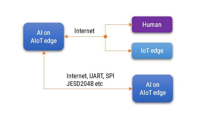
IoT nodes or edge devices use convolutional neural networks (CNN) or neural networks (NN) to perform inference on data collected locally. These devices can include cameras, microphones, or UAV-based sensors. By having the ability to perform inference locally on IoT devices, it enables intelligent communication or interaction with these devices. Other devices involved in the interaction can also be IoT devices, human users, or AIoT devices. This creates opportunities for AIoT (Artificial Intelligence of Things) rather than just IoT, as it facilitates more advanced and intelligent interactions between devices and humans.
- AIoT is interaction with another AIoT. In this case, there is a need for artificial intelligence on both sides to have a meaningful interaction.
- AIoT is interaction with IoT. In this case, there is a need for artificial intelligence on one side, and no AI on the other side. Thus, it is not a good and safe configuration for deployment.
- AIoT is interaction with a human. In this case, there is a need for artificial intelligence on one side and a human on the other side. This is a good configuration because the volume of data from the device to the human will be less.
Human Also in the Loop is a Thing of the Past
Historically, humans have used sensor devices, now referred to as IoT edges or nodes, to perform measurements before making decisions based on a particular set of data. In this process, both humans and IoT edge devices participate. Interaction between one IoT edge and another is common, but typically within restricted applications or well-defined subsystems. With the rise of AI technologies, such as ChatGPT and Watsonx, AI-enabled IoT devices are increasingly interacting with other IoT devices that also incorporate AI. This interaction is prevalent in advanced driver-assistance systems (ADAS) with Level 5 autonomy in vehicles. In earlier terms, this concept was known as Self-Organizing Networks or Cognitive Systems.
The interaction between two AIoT systems introduces new challenges in sensor fusion. For instance, the classic Byzantine Generals Problem has evolved into the Brooks-Iyengar Algorithms, which use interval measurements instead of point measurements to address Byzantine issues. This sensor fusion problem is closely related to the collaborative filtering problem. In this context, sensors must reach a consensus on given data from a group of sensors rather than relying on a single sensor. Traditionally, M measurements with N samples per measurement produce one outcome by averaging data over intervals and across sensor measurements.
Sensor fusion involves integrating data from multiple sensors to obtain more accurate and reliable information than what is possible with individual sensors. By rethinking this problem through the lens of collaborative filtering—an approach widely used in recommendation systems—we can uncover innovative solutions. In this analogy, sensors are akin to users, measurements are comparable to ratings, and the environmental parameters being measured are analogous to items. The goal is to achieve a consensus measurement, similar to how collaborative filtering aims to predict user preferences by aggregating various inputs. Applying collaborative filtering techniques to sensor fusion offers several advantages. Matrix factorization can reveal underlying patterns in the sensor data, handling noise and missing data effectively. Neighborhood-based methods leverage the similarity between sensors to weigh their contributions, enhancing measurement accuracy.
Probabilistic models, such as Bayesian approaches, provide a robust framework for managing uncertainty. By adopting these methods, we can improve the robustness, scalability, and flexibility of sensor fusion, paving the way for more precise and dependable applications in autonomous vehicles, smart cities, and environmental monitoring.
Kalman filtering and collaborative filtering represent two distinct approaches to processing sensor data, each with unique strengths and applications.
Kalman filtering is a recursive algorithm used for estimating the state of a dynamic system from noisy observed measurement data. It excels in real-time applications, offering a mathematically rigorous method of statistically estimating and predicting a model’s state estimates (i.e. a model’s parameters) using a known model of the system’s dynamics and statistical noise characteristics. However, it is important to note that although the ‘Kalman solution’ is optimum in a statistical sense, it may yield incorrect state estimates in a absolute deterministic sense.
In contrast, collaborative filtering, typically used in recommendation systems, aggregates data from multiple sensors (or users) to identify patterns and similarities. This approach doesn’t rely on a predefined model of system dynamics but instead leverages historical data to improve accuracy. Collaborative filtering is particularly effective when dealing with large datasets from multiple sensors, making it suitable for applications where the relationships between sensors can be learned and exploited.
Both methods can enhance sensor data reliability, but their effectiveness depends on the context: Kalman filtering for dynamic, real-time systems with welldefined models, and collaborative filtering for complex, multi-sensor environments where data-driven insights are crucial.
In our AIoT work, we implement Collaborative Filtering across multiple M sensors or AIoT edges to achieve consensus on a measured value over a specified interval. Then use a Restricted Boltzmann Machine (RBM) model for collaborative filtering. Additionally, we deploy and run these types of models within a network of IoT edge devices. This approach leverages the distributed computing capabilities of IoT edges to enhance the performance and scalability of our collaborative filtering solution.
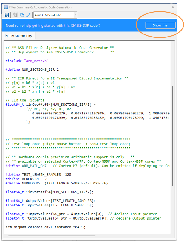
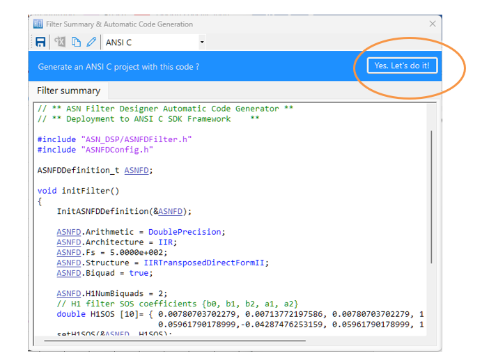
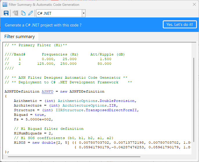
The integration of Collaborative Filtering algorithms with CMSIS (Cortex Microcontroller Software Interface Standard) on Arm devices presents a significant advancement in leveraging edge computing for intelligent decision-making. Collaborative Filtering, commonly used in recommendation systems, can be enhanced on Arm Cortex-M processors by utilizing the CMSIS-DSP library. This combination allows for efficient signal processing and data analysis directly on microcontroller-based systems, enabling real-time and power-efficient computations. This approach can be particularly powerful in IoT applications, where Arm devices often operate. By implementing Restricted Boltzmann Machines (RBM) using CMSIS, devices can process and analyze sensor data locally, reducing latency and bandwidth usage. This local computation capability can lead to more responsive and intelligent IoT systems, paving the way for advanced applications in smart environments, healthcare, and personalized user experiences.
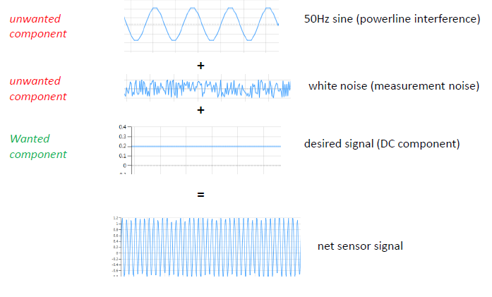
Signal Processing on the IoT edge
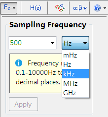
The objective is to measure the signal \(x_n\) for a duration of \(T\) seconds with a sampling rate \(F_s\). The samples collected during that duration \(T\) are \(r_n=1,2,\ldots N\) samples. These measurements are performed \(M\) times repeatedly. Since there are \(M\) sets of \(x_n\) samples of the signal, the revised objective is to find a representative of these \(M\) sets of samples. Let \(\tilde{x}_n \) be the above-mentioned representative.
Let \(y_m(n) = x(n) + v_m(n) \), where \( v_m(n)\) is the measurement noise during the \(m\)-th measurement.
By performing \(M\) measurements, is it possible to
- Improve the Signal to Noise Ratio (SNR)?
- Estimate \(x_n\) using Maximum Likelihood and achieve better performance as per the Cramer-Rao bound?
- Use a priori information about the source that created \(x_n\) and estimate \(x_n\) using a Bayesian network?
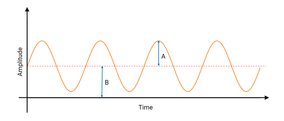
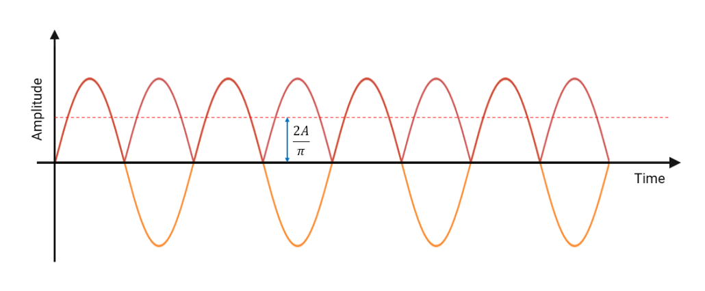
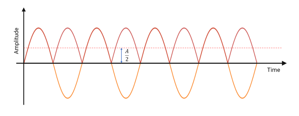
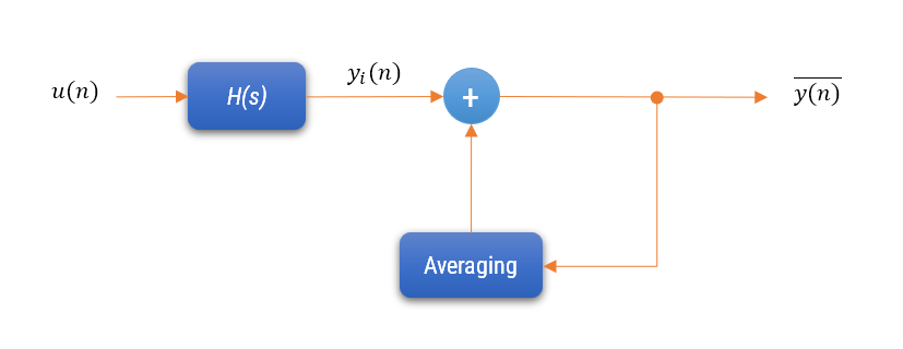
To reduce noise and obtain a more accurate representation of the output signal, multiple measurements of \(y(n)\) are taken over time: \(y_1(n), y_2(n), \ldots, y_M(n) \).
The averaged output signal \(\overline{y(n)} \) is calculated as the mean of these measurements:
\(\displaystyle\overline{y(n)} = \frac{1}{M} \sum_{i=0}^{M-1} y_i(n)\)
Consider a smart thermostat system in a home (part of an AIoT system). The thermostat measures the room temperature \(y(n)\) and adjusts the heating or cooling based on the desired setpoint \(u(n)\).
The following averaging measurement might not yield results that overcome the bounds defined by the Cramer-Rao bound:
\(y_m(n) = x(n) + v_m(n)\)
where \(v_m(n)\) is the measurement noise during the \(m\)-th measurement.
In this context, \(y_m(n) \) represents the noisy measurements of the signal \(x(n)\). Averaging these measurements can reduce the noise variance, but it does not necessarily surpass the theoretical lower bounds on the variance of unbiased estimators, as defined by the Cramer-Rao bound. The Cramer-Rao bound provides a fundamental limit on the precision with which a parameter can be estimated from noisy observations.
- System Description: The thermostat system is represented by \(H(z)\), which controls the heating/cooling based on the input \(u(n)\). The output signal \(y(n)\) represents the measured room temperature.
- Multiple Time Measurements: The thermostat takes temperature measurements every minute, producing a set of outputs \(y_1(n), y_2(n), \ldots, y_M(n)\).
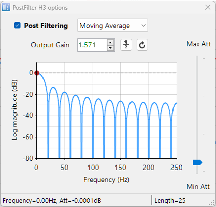
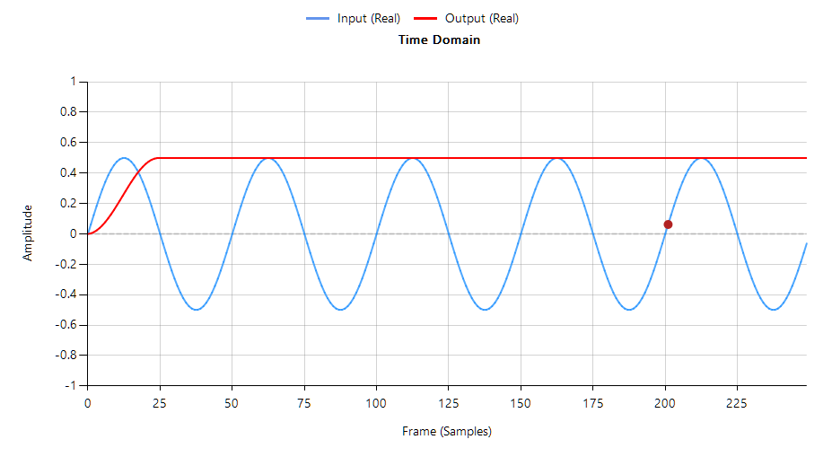
- Averaging: To get a more accurate representation of the room temperature and to filter out noise (e.g., transient changes due to opening a door), the thermostat averages these measurements: \(\overline{y(n)} = \frac{1}{M} \sum_{i=0}^{M-1} y_i(n)\). By averaging the noisy output values \(y_i(n)\), the thermostat system can make more stable and accurate adjustments, leading to a more comfortable and energy-efficient environment.
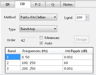
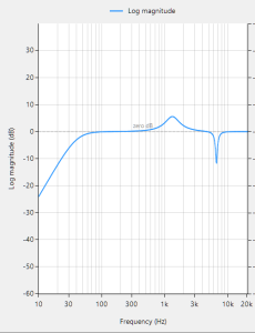
- Latency: One annoying situation that occurs by the averaging operation, is that it increases the system’s latency, i.e. the smoothed output temperature value lags the observed noisy temperature value taken at time n. This delay is referred to as latency or Group delay in digital filters, and must also be taken into account when designing a closed loop control system. The subject of minimising latency in digital filters can fill a whole book in itself, but suffice to say, IIR digital filters generally have lower latency than FIR filters counterparts. The Moving average filter described herein can be considered as a special case of the FIR filter, as all filter coefficients are equal to one.
In order to improve matters, Minimum phase filters (also referred to as zero-latency filters) may be used to overcome the inherent \(N/2\) latency (group delay) in a linear phase FIR filter, by moving any zeros outside of the unit circle to their conjugate reciprocal locations inside the unit circle. The result of this ‘zero flipping operation’ is that the magnitude spectrum will be identical to the original filter, and the phase will be nonlinear, but most importantly the latency will be reduced from \(N/2\) to something much smaller (although non-constant), making it suitable for real-time control applications where IIR filters are typically employed.
AI Model in Signal Processing
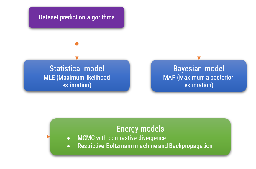
In signal processing, where signals are sensed by sensors, statistical parameterized models, Bayesian networks, and energy models play crucial roles. Statistical parameterized models help in estimating signal parameters efficiently, providing a structured approach to model signal behavior. Bayesian networks offer a probabilistic framework to infer and predict signal characteristics, accommodating uncertainties inherent in sensor data. Energy models, such as those utilizing MCMC with Contrastive Divergence, optimize the representation of signal data by minimizing energy functions, leading to improved signal reconstruction. Similarly, energy models via Restricted Boltzmann Machines and Backpropagation facilitate learning complex signal patterns, enhancing the accuracy of signal interpretation and noise reduction. Together, these models enable robust analysis and processing of signals, crucial for applications like noise reduction, signal enhancement, and feature extraction.
The Cramer-Rao bound (CRB) provides a lower bound on the variance of unbiased estimators, indicating the best possible accuracy one can achieve when estimating parameters from noisy data. This bound applies to traditional estimation methods under certain assumptions, such as unbiasedness and a specific noise model.
MCMC does not directly ‘overcome’ the Cramer-Rao bound, it provides a framework for obtaining parameter estimates that can be more accurate and robust in practice, especially in complex and high-dimensional settings. This improved performance arises from the ability to use prior information, handle complex models, and perform Bayesian inference. Markov Chain Monte Carlo (MCMC) methods, however, are used primarily for sampling from complex probability distributions and performing Bayesian inference. While MCMC methods themselves do not directly ‘overcome’ the CramerRao bound in a traditional sense, they offer advantages in estimation that may be interpreted as achieving better practical performance under certain conditions:
Individual Models
Each model will have ts own bias and variance characteristics. High-capacity models may fit the training data well (low bias) but may perform poorly on new data (high variance). Low-capacity models may underfit the training data (high bias) but have more stable predictions (low variance).
Averaging Models (Ensembles)
By combining the outputs of multiple models, ensemble methods aim to reduce the overall variance. This results in more robust predictions compared to individual models, particularly when the individual models have high variance.
Combining many models seems promising for some applications. When the model capacity is low, it’s difficult to capture the regularities in the data. Conversely, if the model capacity is too large, it may overfit the training data. By using multiple models, such as in AIoT where models can be sensor-centric or device-centric, better results can be achieved compared to using a single huge model.
- High-capacity models tend to have low bias but high variance.
- Averaging models reduces variance, leading to more stable predictions.
- Bias remains unchanged by averaging, so it’s essential to use models with appropriately low bias.
- The ensemble approach can outperform individual models by leveraging the strengths of multiple models, especially in scenarios like AIoT, where combining sensor-centric or device-centric models can lead to improved results.
In some cases, an individual predictor may perform better compared to a combined predictor. However, if individual predictors disagree significantly, then the combined predictor can perform well.
AIoT system building blocks
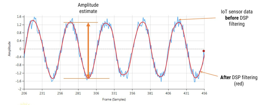
An essential pre-building block in any AIoT system is the feature extraction algorithm. The challenge for any feature extraction algorithm is to extract and enhance any relevant sensor data features in noisy or undesirable circumstances and then pass them onto the ML model in order to provide an accurate classification. The concept is illustrated below:
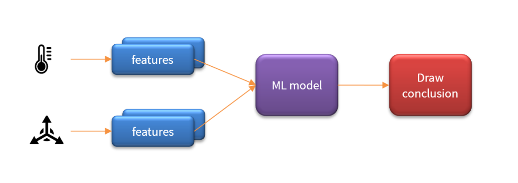
As seen above, an AIoT system may actually contain multiple feature blocks per sensor and in some cases fuse the features locally before sending them onto the ML model for classification such that the system may then draw a conclusion. The challenge is therefore how to capture sensor data for training and design suitable algorithms to extract features of interest?
The challenge is actually two fold: namely how to capture the datasets for analysis and then which algorithms to use for Feature engineering.
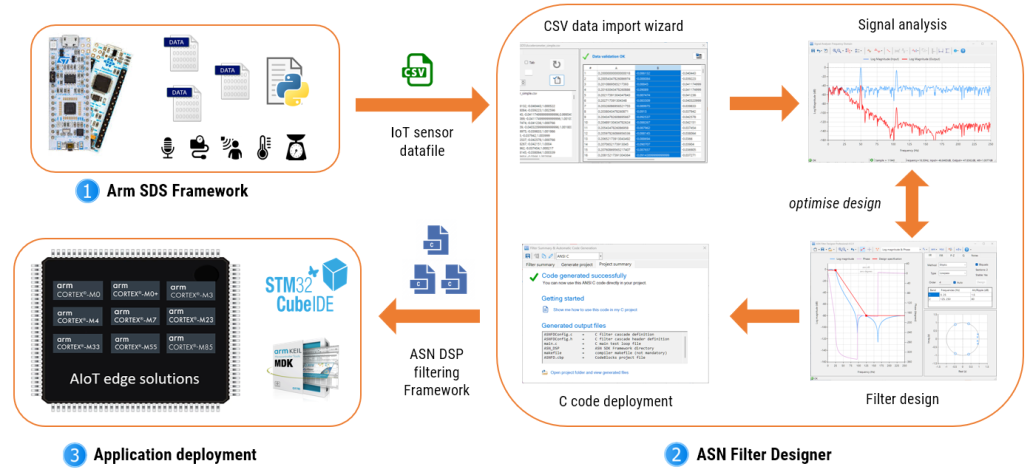
Although a few commercial solutions are available (e.g. Node-RED, Labview, Mathworks Instrumentation toolbox), the latter two are expensive for most developers who just require simple data capture/logging via the UART. One possible solution is Arm’s SDS Framework that provides developers with a set of tools for capturing and playback real-world data using Arm Virtual Hardware. Where, the captured SDS data files can be subsequently converted into a single CSV file for use in 3rd party applications for algorithm development. Unfortunately, the SDS framework is primarily aimed at Arm SoC developers and not particularly suitable for developers working with EVMs/kits.
Therefore, most developers use web tools based on AutoML (eg. Qeexo) that will assist with the data capture from hardware (eg. from an ST Nucleo board) and then try an automate the ML modelling process by choosing a set of limited feature extraction algorithms (such as mean, median, standard deviation, kurtosis etc) and then try and produce a suitable classification model. In theory, this sounds great, but there are a number of problems with this approach, as performance is dependent on the quality and relevance of datasets. Our experience has shown that the best performance can be obtained from knowledge of the physical process, and by designing Feature extraction algorithms using scientific principles tailored to the process that you are trying to model.
Example: Feature Engineering for human fall detection
A common requirement of most IoMT biomedical wearable products is detecting Human fall detection with a smartwatch, just using accelerometer data. Traditional fall detection algorithms using MEMS sensors are based on the ‘Falling’ concept, whereby all three axes fall close to zero for a second or so. Although this works well for falling objects, such as a cup or box falling from a table, it is not suitable for humans. The challenge is illustrated below:
As seen, a human’s fall is very different to a box or other object falling.
The challenge is discriminating between normal everyday activities and falls. By analysing datasets of net acceleration data of typical everyday activities, such as someone walking, using their smartphone, brushing their teeth or doing some morning exercises, and fall data it is not always easy to discriminate between the two using ’standard’ statistical features.
Therefore, we need to apply some physics to the process that we’re trying to model in order to derive specific features from the sensor data, so that we can make a classification – i.e. is it a fall, or not.
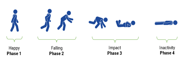
Analysing the diagram we see that there are actually 4 phases from where the person is standing through to the point of the person lying on the ground. So the big question is how do we go about modelling these phases just using accelerometer data? This is best analysed by breaking the fall up into phases:
- Happy: where the subject is upright and going about their daily business.
- Falling: Depending on the subject, this period can be very short (around 100ms) and manifests itself very differently to an object falling directly down (i.e. freefall). The net acceleration will usually manifest itself as a negative gradient starting from about 1g tending towards zero, as the body’s centre of gravity changes. This usually lasts for about 60-100ms.
- Impact: this is the primary event to detect, as any impact from a standing posture with a hard surface will produce a large shock pulse that is several orders of magnitude >1g over a short period.
- Inactivity: this usually follows impact with the ground, whereby the subject is lying flat and is motionless for several seconds. In the case of a collision with an object (e.g. a piece of furniture or a door) or as a result of a severe medical condition, such as a stroke or heart attack, the subject may become unconscious. In this case, the system should be able to discriminate between inactivity from normal movements, such as hand or slight limb movement and light movement (caused by breathing) and decide whether to alert medical services. In the case that no movement is detected, i.e. the subject may have died as a result of the fall, there is no need to provide swift medical assistance.
Armed with this knowledge we can now use Feature engineering to design our features. This forms the essence of building features based on understanding of the physical process.
What tools and processor technology are available?
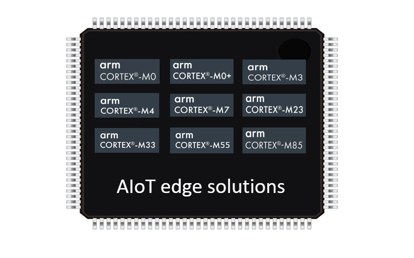
Although a few processor technologies exist for microcontrollers (e.g. RISC-V, Xtensa, MIPS), over 90% of the microcontrollers used in the smart product market are powered by so-called Arm Cortex-M processors. These are split up into various market segments, depending on energy requirements and algorithmic performance.
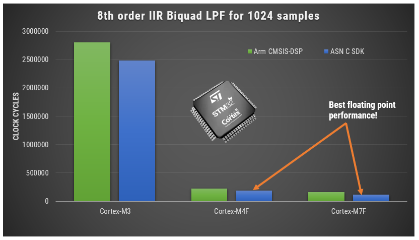
The low-end cores, such as the M0, M0+ and M3 are good for simpler algorithms, such as sensor cleaning filters, simple analytics as they have limited memory and no hardware FP support. To give you an idea of performance, for those of you who own a Fitbit, this is based on the M3 processor.
However, the biggest plus (especially for the M0 family), is that they can have very low power footprint making them an ideal choice for coin cell battery powered wearable applications, as devices can be made to run for months and even in some cases up to a year.
For developers looking for decent computational performance, the M4F is an excellent choice as it has hardware FP support, which is ideal for rapid application development of algorithms. In fact, the Arm Cortex-M4 is a very popular choice with several silicon vendors (including ST, TI, NXP, ADI, Nordic, Microchip, Renesas), as it offers DSP (digital signal processing) functionality traditionally found in more expensive devices and is low-power.
If you need more your application needs more computational performance, then the M7 is an excellent choice, where some devices even offer H/W double precision floating point support, which is ideal for audio enhancement and biomedical algorithms.
For those of you looking for hardware security, then the M33 is a good choice, as it implements Arm TrustZone security architecture, as well as having the computational performance of the M4.
State-of-the art AIoT microcontrollers
Released in 2020, the Arm Cortex-M55 processor and its bigger brother the Cortex-M85 are targeted for AIoT applications on microcontrollers. These processors use Arm’s powerful Armv8.1-M architecture that implement their M-Profile Vector Extension (MVE) technology (nicknamed Helium) allowing for 128bit vector mathematical operations (such as dot product operations) needed for ML and some DSP algorithms.
In November 2023, Arm announced the release of the Cortex-M52 processor for AIoT applications. This processor looks to replace the older M33 processor, as it combines Helium technology with Arm TrustZone technology. However, as only a few IC vendors (Alif, Ambiq, Samsung, Renesas, HiMax, Bestechnic, Qualcomm) have currently released or are planning to release any devices, Helium processors remain a gem for the future.
Toolchains
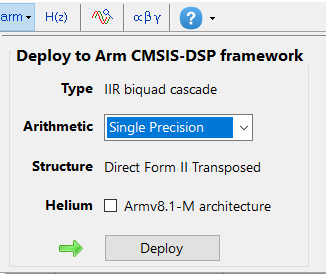
Arm provides developers with extensive easy-to-use tooling and tried and tested software libraries. The Arm’s CMSIS-DSP and CMSIS-NN frameworks for algorithm development and machine learning (ML) are two very popular examples that are open source and are used internationally by tens of thousands of developers.
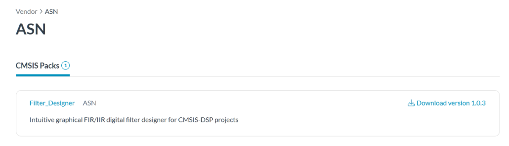
The Arm-CMSIS framework solutions are further strengthened by Arm partners ASN and Qeexo who provide developers with easy-to-use real-time filtering, feature extraction (ASN Filter Designer) and ML tooling (Qeexo AutoML) and reference designs, expediting the development of IoT applications, including industrial, audio and biomedical. These solutions have been optimised for Arm processors with the help of Arm’s architecture experts and insider knowledge of compiler workings.
Deployment of Deep Learning Networks to the IoT Edge
Deploying a trained model onto an Edge device requires meticulous attention and effort. Fortunately, there are many tools available to help developers achieve this, such as Qeexo AutoML and the DLtrain toolset. The latter offers robust support for developers working with Arm processor-based boards with Android platforms. DLtrain utilizes the Android NDK (native development kit) to deploy neural networks (NN) or convolutional neural networks (CNN) in the Linux kernel of the Android platform. The deployed components include JNI options to support applications developed in Java, bridging the gap between low-level implementation and high-level application development. Find out more here.
Deploying deep learning (DL) networks on Arm cores of Android platforms involves integrating these networks into the Linux kernel via the Android NDK. While application development is primarily done in Java, DL networks receive input from the Android layer (SDK) and efficiently perform inference. The results are then passed back to the Java side via the Java Native Interface (JNI). The following list describes the layers involved in performing inference on an Android device:
- Top Layer: User Interface
- Second Layer: Java
- Third Layer: Android SDK
- Fourth Layer: Arm
- Bottom Layer: GPU
This hierarchical structure ensures that the user interface seamlessly interacts with underlying DL networks, optimizing performance and maintaining an efficient workflow from input to inference to output.
Key takeways
AI is an umbrella term focused on creating intelligent systems, whereas ML is a subset of AI that involves creating models to learn from data and make decisions. ML is crucial for IoT because it enables efficient data analysis, predictive maintenance, smart automation, anomaly detection, and personalized user experiences, all of which are essential for maximizing the value and effectiveness of IoT deployments.
Arm and its rich ecosystem of partners provide IoT developers with extensive easy-to-use tooling and tried and tested software libraries for designing an implementing IoT algorithms for their smart products. Arm Cortex-MxF processors expedite RAD by virtue of their ease of use and hardware floating-point support, and modern semiconductor technology ensures low-power profiles making the technology an excellent fit for IoT/AIoT mobile/wearables applications.