Baseline wander (BLW) is one of the most persistent — and misunderstood — problems in ECG systems. Caused by respiration, movement, and electrode drift, BLW introduces low-frequency drift that can distort key waveform features and disrupt clinical analytics.
While BLW suppression is essential and mandated in all ECG systems, developers often face two key challenges:
- Interpreting the filtering requirements in standards such as IEC 60601-2-25 and 60601-2-47, which define passband specifications but fall short on practical implementation guidance
- Designing real-time, morphology-preserving filters that are efficient enough to run on embedded platforms such as modern low power microcontrollers used in modern wearable and portable devices.
In both the United States and Europe, regulatory bodies reference the IEC 60601-2-25 and 60601-2-47 standards when evaluating ECG systems. In the United States, the FDA uses them as a key part of its review process, while in Europe they form the basis for CE marking under the MDR (Medical Device Regulation, EU 2017/745). As such, adhering to IEC 60601-2-25 and 60601-2-47 is essential for global regulatory compliance.
Despite the growing use of AI and ML in ECG signal processing, current IEC and FDA standards have not yet caught up. There is no formal guidance on how to validate AI-based filtering or classification pipelines, leaving developers without a clear compliance path when using these emerging techniques.
As a result, most developers still rely on traditional digital filtering methods — especially when targeting regulatory approval. This is particularly true in wearable and portable devices, where Arm Cortex-M microcontrollers, such as the STM32 family, are the dominant hardware platform. Yet even here, many continue to follow legacy filtering advice inherited from the analog era, without re-evaluating what’s truly required for today’s real-time digital systems.
In this article, we break down what the standards actually require, explaining where the widely-cited 0.05 Hz cutoff comes from, and show how to design real-time high-pass filters that balance signal quality, compliance, and power efficiency — all within the constraints of modern embedded platforms such as the STM32 microcontroller.
What the standards don’t say, and why this is confusing
While IEC 60601-2-25 and IEC 60601-2-47 do define passband requirements (e.g., 0.05–150 Hz or 0.67–40 Hz), but they don’t offer practical engineering guidance for how to meet those requirements on resource-constrained platforms like wearables.
They don’t cover things such as:
- How to implement the filter in a real-time embedded system
- Trade-offs between FIR vs IIR in morphology-sensitive signals
- What to do about SoCs with built-in analog filtering
- Energy/performance implications of filter design choices
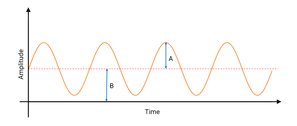
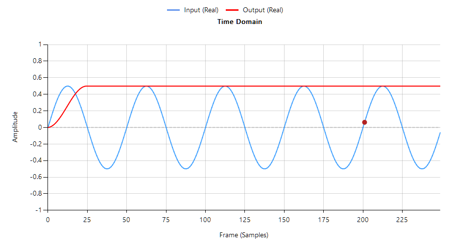
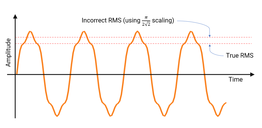
- How to practically validate the signal chain for compliance — e.g. when conducting the ‘sinewave test’, should the amplitude of the 0.67-40Hz test sinewaves be measured continuously or averaged over time? Should I use RMS or peak amplitude when comparing the amplitudes with the 5Hz reference amplitude?
This leaves engineers with many unanswered questions:
- Is a 0.05 Hz cutoff always necessary?
- What level of phase distortion is acceptable?
- Can I use an IIR filter and still be compliant?
- How do I qualify an SoC with undocumented internal filters?
- What measurement methodology should I use for compliance testing?
As a result, developers often either overdesign their filters based on worst-case diagnostic assumptions — or under-design, thinking any high-pass filter will suffice. Neither approach guarantees compliance or robust signal quality.
Baseline wander (BLW) is a well-known issue in ECG systems, arising from slow movements such as respiration, torso motion and electrode impedance shifts. As a consequence, BLW introduces a low-frequency drift, distorting the ECG baseline and compromising the accuracy of QRS detection, HRV analysis, and waveform interpretation.
While baseline wander (BLW) suppression is essential — and mandated in all ECG systems, developers often face two key challenges:
- Interpreting the filtering requirements in standards such as IEC 60601-2-25 and 60601-2-47, which define passband specifications but fall short on practical implementation guidance
- Designing real-time, morphology-preserving filters that are efficient enough to run on embedded platforms such as modern low power microcontrollers
These issues often lead to overengineered solutions, misinterpretation of compliance requirements, or filters that distort clinically relevant features — all of which can compromise both product performance and regulatory approval.
0.05 Hz: A Diagnostic-Grade requirement from IEC standards
The 0.05 Hz lower cutoff frequency originates from IEC 60601-2-25, which governs diagnostic electrocardiographs. It is also referenced in IEC 60601-2-47 for ambulatory ECG systems when high-fidelity diagnostic performance is required.
The mandated system bandwidth of 0.05-150 Hz is intended to preserve:
- ST-segment deviations
- T-wave alternans and morphology
- Other slow-changing diagnostic features
This specification is well-suited to clinical and hospital environments but presents serious challenges for embedded systems.
Why 0.05 Hz is difficult to implement in realtime
To meet this requirement, developers usually consider two filtering options:
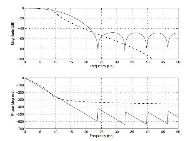
- IIR filters: These are computationally efficient but exhibit non-linear phase response, causing phase distortion that alters the shape of the QRS complex. This makes IIR filters unsuitable for ECG applications where signal morphology is critical.
- FIR filters with linear phase: These preserve morphology but require very long filter lengths—often extending to 5-10k filter coefficients for a 0.05 Hz cutoff—resulting in increased memory use, latency, and computational cost.
Choosing the best cut-off frequency
Wearable ECG systems operate under constraints in power and processing. These systems typically target a bandwidth of 0.5-40 Hz. This is sufficient for preserving the key features of the ECG waveform, while also easing implementation on embedded hardware. This range aligns with reduced fidelity requirements in IEC 60601-2-47 for wearable or monitoring devices.
Where does BLW actually occur?
In practice, the majority of BLW energy is concentrated below 0.5 Hz. This is supported by:
- Real-world ECG datasets
- Clinical literature on motion and respiration artefacts
- Empirical testing using wearable sensors under normal conditions
Sources of BLW such as respiration (~0.2–0.3 Hz), slow body movement, and electrode drift typically lie in the <0.5 Hz region. This means: a high-pass filter with a cutoff of 0.5 Hz or 0.67 Hz will suppress most baseline drift without distorting the QRS complex or T-wave morphology.
This insight is essential for wearable and mobile ECG systems, where developers must balance:
- Signal fidelity
- Computational efficiency
- Power consumption
- Compliance with IEC 60601-2-47 (where applicable)
Over-filtering (e.g., using a 1 Hz high-pass cutoff) can begin to distort critical ECG features, particularly the ST segment and T-wave. On the other hand, under-filtering may leave residual baseline drift that impacts analytics such as heart rate variability and R-peak detection.
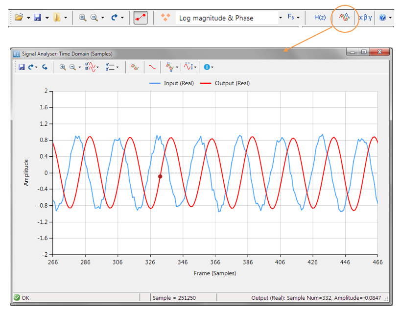
The following animation demonstrates how the QRS is warped when using a 1st order IIR filter.
The 0.5–0.67 Hz cutoff range is often the optimal balance in wearable ECG systems — effective in suppressing baseline wander while preserving essential waveform morphology.
In fact, IEC 60601-2-47 stipulates that a 0.67Hz cut-off may be used if no phase distortion is introduced. We can therefore conclude that a signal bandwidth of 0.67-40Hz is IEC compliant for ambulant systems.
When implemented with a linear-phase FIR filter, this approach meets both signal quality and regulatory requirements — and remains computationally feasible for embedded targets such as the STM32.
Implementation on STM32 microcontrollers
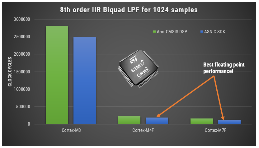
STM32 microcontrollers built on the Arm Cortex-M architecture (e.g. M4, M7 cores) are a popular choice for wearable ECG systems. They offer a solid combination of processing performance, on-chip memory, and energy efficiency — all critical factors for medical-grade real-time signal processing.
When implementing high-pass filters for baseline wander suppression, several hardware and algorithmic factors must be considered:
- Hardware Floating-Point Support expedites RAD: devices like the STM32F4, F7, and H7 feature single-precision floating-point units (FPUs). This allows developers to expedite RAD (rapid application development) by prototyping and validating filters quickly without needing to deal with fixed-point scaling and rounding errors.
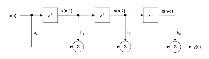
- FIR Filters preserve morphology, but are computationally heavy: Linear-phase FIR filters are strongly recommended for ECG applications because they preserve temporal relationships of the waveform, which is essential for correct analysis.
However,
- A 0.5 Hz cutoff at 200 Hz sampling typically requires 100s of filter coefficients, which is manageable on most STM32 devices (Cortex-M4/M7), and just about manageable on ultralow power Cortex-M0+ devices.
- In contrast, a 0.05 Hz cutoff typically requires 1000s of filter coefficients (10k+ in some cases), resulting in high memory usage and processing load — often beyond what’s practical for real-time wearable designs.
- A 0.5 Hz cutoff at 200 Hz sampling typically requires 100s of filter coefficients, which is manageable on most STM32 devices (Cortex-M4/M7), and just about manageable on ultralow power Cortex-M0+ devices.
- Affect on battery life: Long FIR filters keep the FPU active nearly continuously, which prevents the microcontroller from entering low-power states. This significantly impacts battery life — especially in wearables running at higher sample rates, e.g. 500 Hz. For this reason, the cutoff frequency must be carefully selected to balance signal quality with energy efficiency.
- Avoid IIR Filters for morphology-critical Applications: While IIR filters are computationally attractive due to their low order, they introduce non-linear phase distortion. This warps the QRS complex, alters timing relationships between ECG segments, and undermines compliance with medical waveform standards. For any application where waveform shape matters, IIR filters should be avoided.
Ultimately, for wearable ECG systems targeting compliance and signal integrity, linear-phase FIR filters on STM32 microcontrollers provide the most practical and reliable foundation for real-time baseline wander removal.
Multirate FIR Filtering for computationally efficient ECG filtering
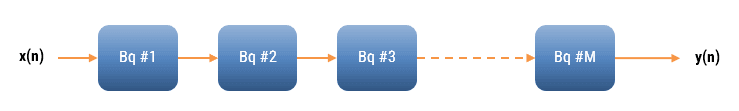
FIR filter cascades are among the most practical and precise methods for implementing baseline wander removal, particularly when combined with decimation and multirate techniques. Baseline wander removal using FIR filters can be implemented in two primary ways: by cascading multiple FIR low-pass filters and subtracting the result from the original signal, or by designing a cascade of high-pass FIR filters directly. Both approaches are suitable for use in systems that must preserve ECG morphology, with the subtraction method offering particularly clear control over the high-pass behaviour when combined with multirate stages.
This approach offers a high degree of flexibility, as the designer can control the cutoff frequency, stopband attenuation, and transition width with great precision. It also supports linear-phase operation, ensuring that waveform features like the QRS complex remain undistorted — a crucial factor for diagnostic applications.
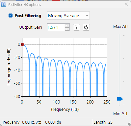
Although other techniques exist — such as moving average filters and the Kolmogorov-Zurbenko (KZ) cascade, which is a cascade of identical moving average filters — these methods are computationally efficient and linear-phase by nature, but they lack the precise frequency shaping and design flexibility that FIR filters provide. FIR-based filtering, by contrast, gives developers precise control over the cutoff, transition width, and stopband characteristics — making it a strong choice for applications where accurate control over the frequency characteristics are required — particularly in systems targeting regulatory compliance.
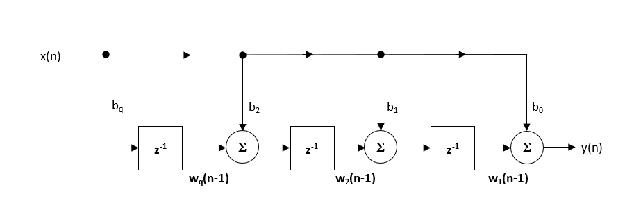
FIR filters can also be optimized using polyphase decomposition, which restructures the filter to operate only at decimated output points. This avoids unnecessary computation and memory access, especially when combined with multistage decimation, where each FIR stage operates at a lower sampling rate than the previous one. Instead of a single large filter at the original sampling rate, several short FIRs operating at lower rates achieve the same result with far fewer operations per second.
Even though Cortex-M processors like the STM32F4/F7 lack true parallelism, the polyphase structure maps efficiently onto SIMD instructions, improving throughput and reducing power consumption. FIR filtering, when designed with multirate and polyphase techniques, provides a scalable and standards-compliant solution for real-time baseline wander removal on embedded platforms.
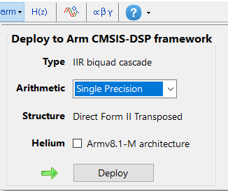
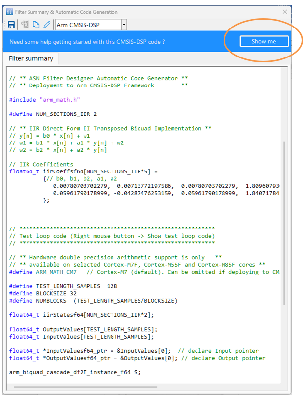
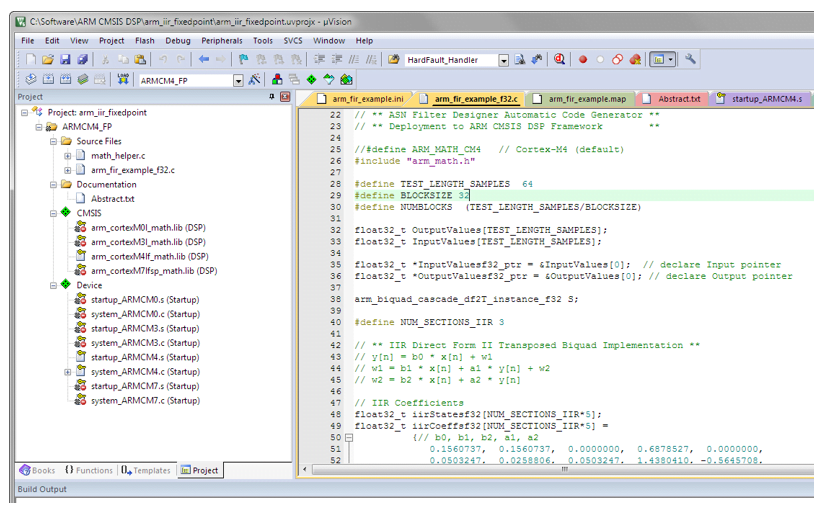
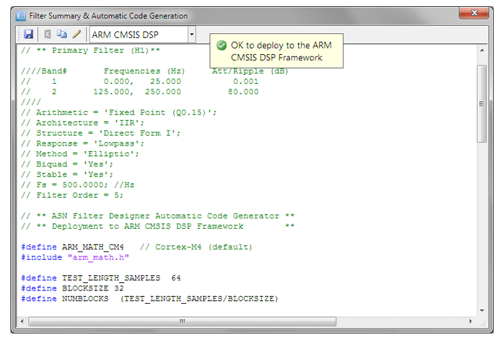
The following C code snippet uses the Arm CMSIS-DSP framework to implement an FIR filter designed for a 0.05 Hz high-pass cutoff, assuming the signal is decimated from 200 Hz to 20 Hz. The decimation factor of 10 significantly reduces the computational load, making a long FIR filter more practical for embedded systems.
#include "arm_math.h"

#define BLOCK_SIZE         200   // Number of input samples per call
#define NUM_TAPS           120   // FIR filter length designed at 20 Hz sampling rate
#define DECIMATION_FACTOR  10    // Decimate by 10 (200 Hz → 20 Hz)

// FIR coefficients designed offline for 0.05 Hz high-pass at 20 Hz
extern float32_t firCoeffs[NUM_TAPS];

float32_t firState[BLOCK_SIZE + NUM_TAPS - 1];
float32_t inputBuffer[BLOCK_SIZE];
float32_t outputBuffer[BLOCK_SIZE / DECIMATION_FACTOR];

arm_fir_decimate_instance_f32 S;

// Initialization
arm_fir_decimate_init_f32(&S, NUM_TAPS, DECIMATION_FACTOR, firCoeffs, firState, BLOCK_SIZE);

// Processing loop
arm_fir_decimate_f32(&S, inputBuffer, outputBuffer, BLOCK_SIZE);
As a closing remark, it’s certainly true that many developers — especially in research or offline processing environments — use zero-phase IIR filtering by applying the filter forward and backward through the signal. While this technique avoids phase distortion and preserves waveform morphology, it is inherently non-causal and unsuitable for real-time applications. This distinction is critical, as filters that rely on forward-backward (zero-phase) processing cannot be implemented in real-time embedded systems, making them unsuitable for wearable applications that operate on streaming data.
Biomedical SoCs: Powerful, but require full signal-chain qualification
Several IC vendors — including Analog Devices (ADI), Texas Instruments (TI), and STMicroelectronics — have developed highly integrated biomedical SoCs that feature built-in analog front ends (AFEs). These devices often include:
- Programmable gain amplifiers
- Instrumentation amplifiers
- Integrated analog filtering
- High-resolution ADCs with CIC (Cascaded Integrator-Comb) filters
While these SoCs offer impressive integration and are well-suited for compact, low-power designs, they also introduce a significant challenge, i.e. Developers must still qualify the entire signal chain — including analog and digital filter stages — to ensure IEC compliance.
Typical challenges include:
- Measuring the overall frequency response of the signal path
- Evaluating the effects of CIC decimation filters and analog high-pass/low-pass stages
- Understanding the behaviour of any hidden gain or filtering elements inside the AFE or ADC
Because much of this behaviour is not fully documented, it often requires empirical validation using signal injection and sweep testing — a tedious and time-consuming process that many teams underestimate.
Without this validation, there’s a real risk of:
- Non-compliant frequency response
- Undetected distortion of QRS or ST segments
- Unexpected interaction between analog filtering and digital signal processing
Bottom line: integrated SoCs are powerful, but compliance is never automatic. It’s up to the developer to fully characterize and correct the signal path to meet the requirements of IEC 60601-2-47 — especially when targeting diagnostic or screening-grade wearable ECG systems.
Recommendations based on legacy systems
The commonly referenced 0.05 Hz high-pass cutoff originates from the behaviour of first-order analog filters used in ECG systems developed in the 1970s and 1980s. These filters had slow roll-off and introduced significant phase distortion, but were accepted at the time due to the limitations of analog circuitry and minimal awareness of morphology distortion effects.
Over time, this cutoff value was incorporated into standards such as IEC 60601-2-25, and later IEC 60601-2-47, often without re-evaluation in the context of modern digital systems. As a result, much of today’s ECG design guidance continues to reflect analog-era limitations, despite dramatic advances in hardware and signal processing.
It’s also worth noting that much of the legacy design advice found in textbooks and reference designs stems from the ‘analog era’ — when discrete op-amps, analog filters, and limited processing power dictated system architecture. While those principles served their purpose, modern biomedical SoCs and real-time digital filtering pipelines operate under entirely different constraints and possibilities.
As a result, engineers must challenge inherited assumptions, revalidate their signal path in the digital domain, and adopt design practices suited to real-time embedded systems — not outdated analog models.
This shift in mindset is essential not only for meeting IEC compliance in modern systems, but for achieving robust, efficient, and clinically reliable signal quality — especially in wearable and low-power applications.
Designing for Clarity, Compliance and Real-time constraints
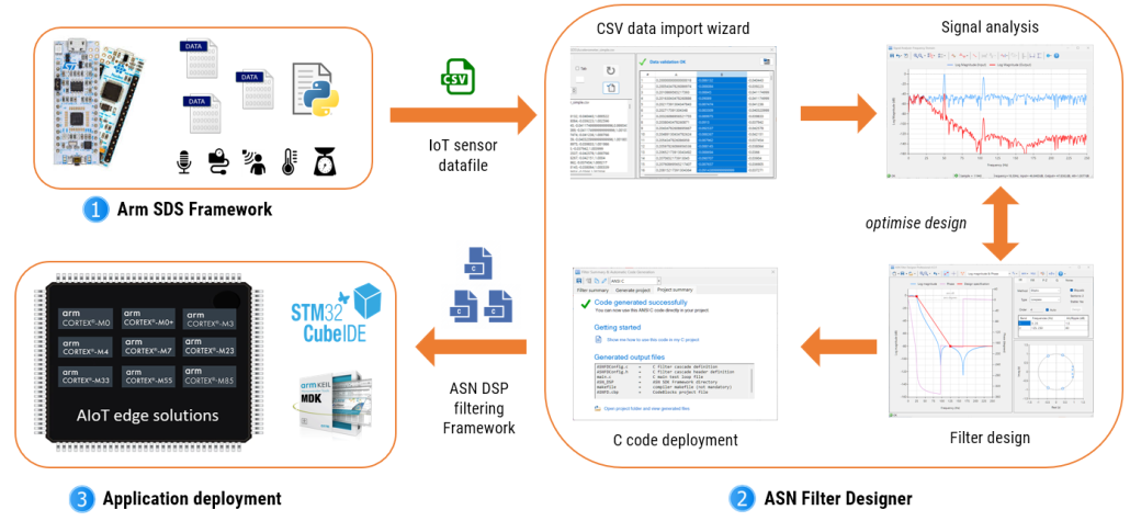
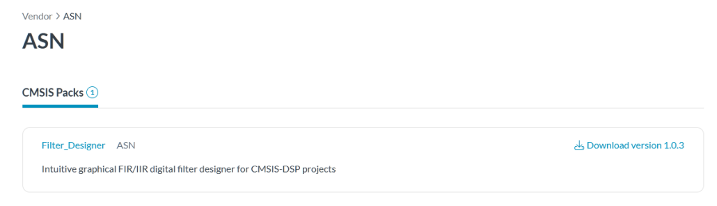
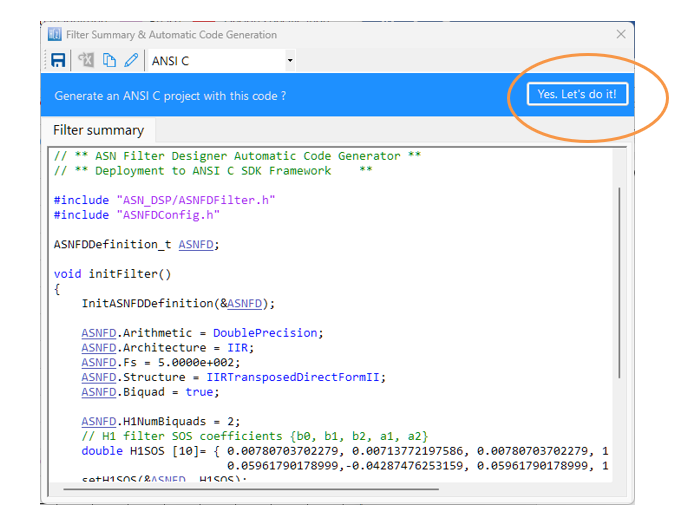
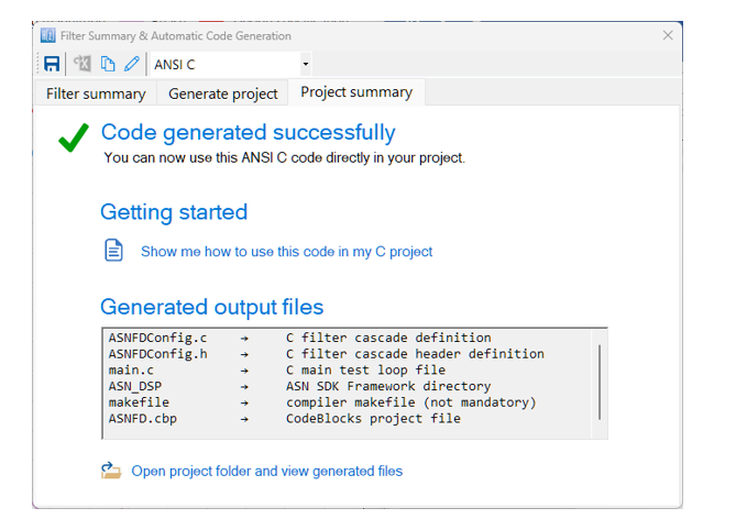
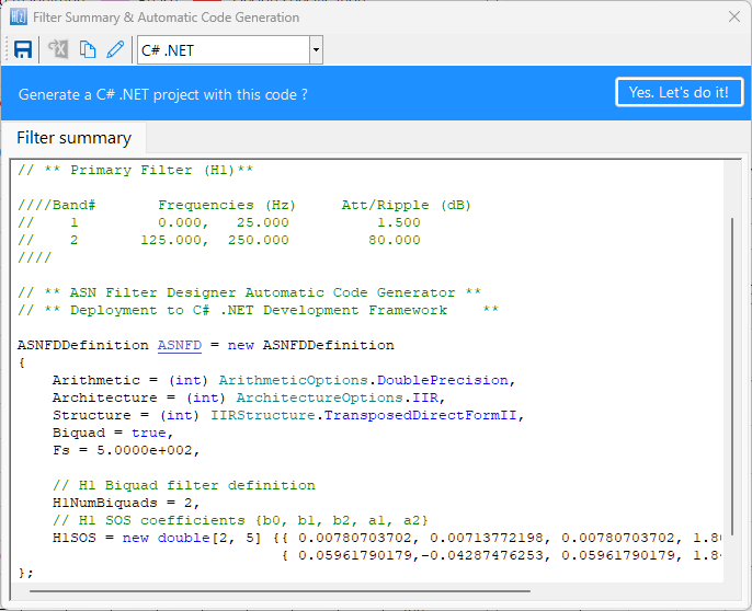
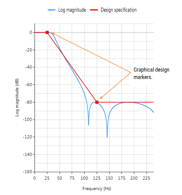
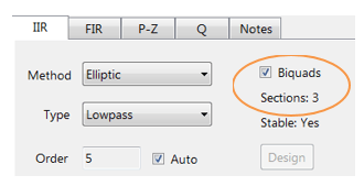
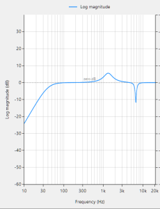
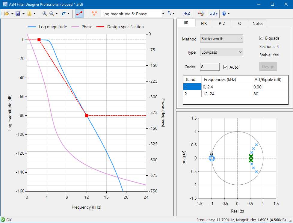
Tools such as the ASN Filter Designer simplify ECG filter development by providing:
- Reference designs for designing linear phase IEC compliant ECG filter cascades (0.5-40Hz)
- High accuracy frequency response charts
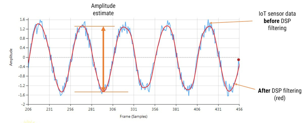
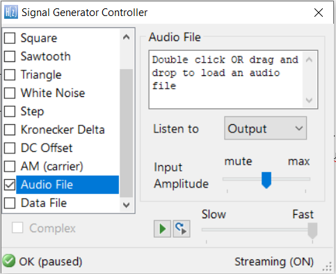
- The ability to load and stream ECG dataset to visualize filter performance in real-time
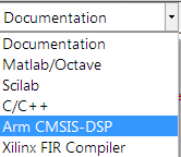
- Code export options for Arm processors (ANSI C) and Python and Matlab
This allows engineers to deploy real-time, medically robust filters quickly and with confidence.
Key Takeaways
A 0.05 Hz high-pass cutoff is referenced in both IEC 60601-2-25 (diagnostic ECG) and IEC 60601-2-47 (ambulatory ECG) for systems intended to support full diagnostic fidelity. However, this requirement is not appropriate for most wearable applications.
In wearable environments, baseline wander is dominated by motion and respiration artefacts, most of which lie below 0.5 Hz. As such, filtering at 0.05 Hz does not sufficiently suppress BLW, and imposes significant implementation burdens — including high memory usage, increased latency, high computation requirements and greater power consumption.
Crucially, IEC 60601-2-47 permits a high-pass cutoff of 0.67 Hz for ambulatory systems, provided that no phase distortion is introduced. When implemented using a linear-phase FIR filtering, a bandwidth of 0.67–40 Hz is both IEC-compliant and technically practical for real-time implementation on embedded platforms such as the STM32.
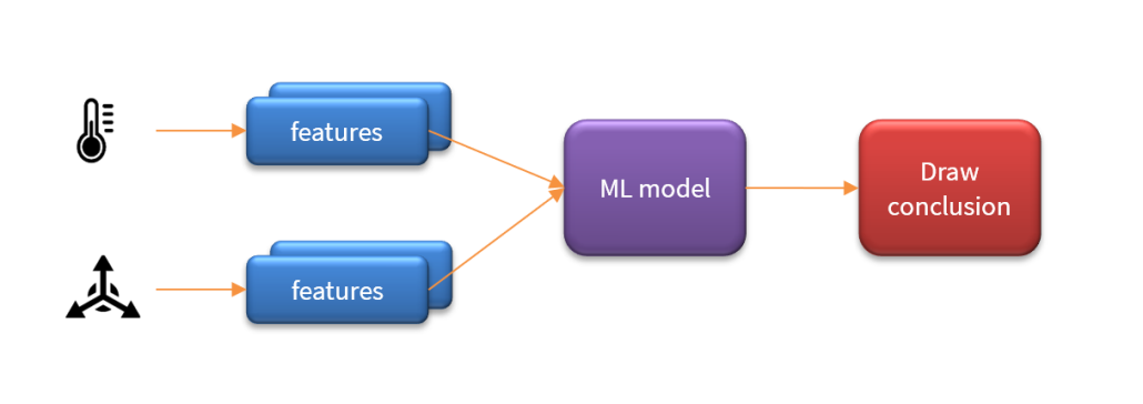
AI-based ECG processing
While the current standards, including IEC 60601-2-47, provide guidance for traditional digital filtering approaches, it’s important to note that they have not yet caught up with AI-based ECG processing techniques. As of today, there are no formal standards, validation protocols, or compliance pathways defined for ECG systems using AI/ML for baseline correction or morphology analysis.
This lack of regulatory clarity means that, for now, classical digital filtering — particularly linear-phase FIR filters — remains the most robust, transparent, and standards-aligned approach for ensuring ECG signal quality and achieving IEC/FDA compliance in wearable and ambulatory systems.
ASN Solutions and Expertise
At ASN, we’ve supported numerous international clients in designing medically robust ECG systems — including helping them achieve FDA and IEC 60601-2-47 compliance. From real-time FIR filter design to signal chain validation and compliance testing workflows, we offer practical, implementation-ready solutions tailored for modern embedded systems and wearable applications.